Scene analysis for effective visual search in rough three-dimensional-modeling scenes

Qi Wang; Xiaopeng Hu

doi:10.1117/1.JEI.25.6.061622

20 December 2016 Scene analysis for effective visual search in rough three-dimensional-modeling scenes

Qi Wang, Xiaopeng Hu

Author Affiliations +

Journal of Electronic Imaging, Vol. 25, Issue 6, 061622 (December 2016). https://doi.org/10.1117/1.JEI.25.6.061622

Abstract

Visual search is a fundamental technology in the computer vision community. It is difficult to find an object in complex scenes when there exist similar distracters in the background. We propose a target search method in rough three-dimensional-modeling scenes based on a vision salience theory and camera imaging model. We give the definition of salience of objects (or features) and explain the way that salience measurements of objects are calculated. Also, we present one type of search path that guides to the target through salience objects. Along the search path, when the previous objects are localized, the search region of each subsequent object decreases, which is calculated through imaging model and an optimization method. The experimental results indicate that the proposed method is capable of resolving the ambiguities resulting from distracters containing similar visual features with the target, leading to an improvement of search speed by over 50%.

1. Introduction

Visual search is one of the critical technologies in the field of computer vision; it can support high-level applications such as motion analysis, image understanding, and so on. It is a common task to find specific objects in the scene that have been roughly three-dimensional (3-D) modeled by methods such as simultaneous localization and mapping (SLAM)¹ or structure from motion (SFM).² In these scenarios, location information can be supplied by sensors such as global position system in the outdoors or RGB-D in the indoors. Corresponding 3-D-coordinates of some image pixels can be calculated by triangulation methods.³ For this case, we refer to rough 3-D-modeling scenes.

The specific target is usually hard to discover owing to complex natural scenes that contain similar distracters. A feasible way to find the specific target is through the positions of the salient objects in the same scene. Intuitively, given a known point in the rough 3-D-modeling scenes, the search region in the image of the target will be decreased. In this paper, we build an optimization model for this issue based on a camera imaging model. Through this optimization method, we calculate the search regions of the other points when a two-dimensional (2-D)–3-D point pair is found. Brief reviews about camera imaging models are depicted in Sec. 3.2.1.

The salience computation model was first proposed by Itti et al.⁴ Until now, Itti’s model was still competitive with current state-of-the-art methods.⁵ In Itti’s model, salience measurements of visual features are computed according to the local contrast principle. Then, the salience values are sorted in descending order. Finally, a visual search path of features is formed. Itti’s salience model and the subsequent improved methods focus on salient object detection or fixation prediction.⁶ In this type of search path formed by these methods, features are independent from each other and relations of features are not taken into account. By those methods mentioned in Ref. 6, the nonsalience objects cannot be found according to their salience estimation. Actually, relations exist among visual features, which are confirmed in Ref. 7. In this paper, our salience model is designed so that the salience measurement is computed with respect to the search region. Features can be analyzed quantitatively in the specific search region. The search region is decreased if a salient feature is found in rough 3-D-modeling scenes. In the decreased search region, nonsalient objects can become salience and be localized.

We propose a visual search method based on vision salience theory and a camera imaging model, which performs rapid and accurate object locating along a visual search path. This search path takes account of the relations of visual features. Consider the problem that we want to find the coin in the dot line circle, as shown in Fig. 1, which contains the colinear key and battery, the cluster of coins, and so on. If we seek the coin in the whole image by the traversal algorithm, it is inefficient and easily affected by clutter like similar objects. However, we will carry out the visual search along the path as follows: first, the key in the solid line circle; second, the button cell in the dash line circle; and last, the coin in the dot line circle. At each step, we actually detect the salient object in the given region. More notably, the search region of each object along the path is decreased gradually. Owing to the operations of this model, we can (i) estimate the saliency of features in the given search region; (ii) eliminate the effect of similar distracters in the background; and (iii) decrease the search region to improve the salience of features.

Fig. 1

An example of search path. The target is the coin in the dot line circle. The search path is composed as follows: first, the key in the solid line circle; second, the button cell in the dash line circle; and last, the coin in the dot line circle.

There are six sections in this paper. In Secs. 1 and 2, we give the introduction and related works. In Sec. 3, first we introduce the definitions of saliency and search path used in this paper. The two concepts instruct how to find the specific object. Second, we present the method of how to calculate the search region of features along the search path. We illustrate how a feature that has been found affects the subsequent features along the path according to the optimization model. Third, we describe the whole algorithm process. Details of the algorithm reveal the formulation of a search path that arrives at the final target. In Sec. 4, we give the experiments to demonstrate the effectiveness of our method. In Secs. 5 and 6, we propose some directions for future work and conclude our paper.

2. Related Works

Saliency is an important part of the overall process of lots of applications. Recently, researchers attempted to learn and utilize human visual search to guide salience computational mechanism.⁸^,⁹ In Itti’s model, saliency of visual features is computed by means of center-surround mechanism, which is an implementation of local contrast. Information theory, Bayesian inference, graphical models, and so on are also introduced to represent local contrast and calculate saliency by other researchers. Bruce and Tsotsos¹⁰ presented a salience model in which self-information of local image patch is used to determine the salience measure. Hou and Zhang¹¹ utilized incremental coding length to select salient features with the objective to maximize the entropy across sample features. Li et al.¹² defined the saliency as the minimum conditional entropy given the surrounding area. The minimum conditional entropy is further approximated by the lossy coding length of Gaussian data. Butko and Movellan¹³ built probabilistic models of the target, action, and sensor uncertainty, and used information gain to direct attention to a new location. Gao et al.¹⁴ considered the discriminant saliency as a one-versus-all classification problem in which kullback-leibler divergence is used to select salient features. Zhang et al.¹⁵ presented a Bayesian model to incorporate contextual priors in which the overall saliency is computed by the pointwise mutual information between the features and the target. Harel et al.¹⁶ presented a fully connected graph over all pixels, which is then treated as a Markov chain to obtain the salience value. Chikkerur et al.¹⁷ designed a Bayesian graph model that combines the spatial attention and feature-based attention.

However, research on the salience computational model is still in a fledging period. Most work, including the methods aforementioned, concentrates on using or modifying the salience model proposed by Itti et al.⁶ because all saliency systems can be seen as a local contrast computation model.⁵ Computing local contrast is an essential step for saliency estimation.⁵ Whether objects are salience or not is determined by their difference from the surrounding area. Given the surrounding area, the methods aforementioned are only designed to produce static salience estimation. Relations of features beyond the appointed local scope cannot be taken into an account. As a result, the salience estimation cannot provide evidence to locate nonsalient objects. Our method is still based on local contrast; however, we calculate the local contrast of features by making use of the search region. The search region can be computed dynamically to improve the salience of features.

3. Method Formulation

In this section, we describe the details of our method and propose an algorithm that generates a search path guiding to the target. In this paper, the following notations are required to describe a 3-D scene.

3.1.

Region-Based Salience Analysis

In this paper, we take advantage of the visual search mechanism to find the salient objects preferentially, so we can improve the search speed and accurate rate. First of all, we give the definition of the salience of objects used in our paper and the method how to calculate it.

Definition 1.

Given scene image $I$ , search region $Ω$ , and feature $f$ , the salience measurement of object $O_{k} \in Ω$ with respect to $I$ , $Ω$ , and $f$ is

Eq. (1)

L (O_{k} | I, Ω, f) = \min_{O_{j} \in Ω, O_{j} \neq O_{k}} [\frac{P (f | O_{k}, I)}{P (f | O_{j}, I)}] = \frac{P (f | O_{k}, I)}{\max_{O_{j} \in Ω, O_{j} \neq O_{k}} P (f | O_{j}, I)} .

Given scene image $I$ , search region $Ω$ , feature $f$ , and threshold $η$ , $O_{k}$ is a salience object, indicated by $S (O_{k} | I, Ω, f, η)$ , with respect to region $Ω$ if and only if

Eq. (2)

L (O_{k} | I, Ω, f) \geq η .

Threshold

η

is determined by detection rate.

In Definition 1, we define the salience of objects with the method of Bayesian maximum likelihood. For example, $N$ similar features are located in the same search region. The salience measure of a specific feature $f$ is $L = \frac{1 / N}{(N - 1) / N} = \frac{1}{N - 1}$ . If feature $f$ is unique, i.e., $N = 1$ , the salience measure of $f$ is the defined max value. On the contrary, the salience measure of $f$ will become small. Compared with common objects, salience objects are more discriminable and different from their background. As a result, they can be detected with a higher accuracy rate.

Definition 2.

Given scene image $I$ , a target $O$ is searchable if and only if

a. there exists a search region and feature so that $O$ is a salience object;
b. there exists a search path so that $O$ is reachable.

According to Definition 2, the search process proceeds along a path composed of salient object → salient object →⋯→ target. The search path performs the target search through locating salient objects step by step. In this search path, the closer to the target, the smaller the search regions of the salient objects become. Areas of search regions are determined by the previous found features, which are depicted in Sec. 3.2. Through such operations, we can make use of relations among features.

Proposition 1.

Given scene image $I$ , search region $Ω_{1}$ and $Ω_{2}$ , feature $f$ , and object $O$ , we have

Eq. (3)

S (O | I, Ω_{1}, f, η) \land Ω_{2} \subseteq Ω_{1} \land O \in Ω_{2} \Rightarrow S (O | I, Ω_{2}, f, η) .

Proposition 1 shows that in a shrunken region salient object is still salience. This proposition guarantees that we can determine a salient object in a large region. As a result, the effect from the previous features, which makes the region shrink, can be utilized correctly. Each node of this path confirms the position of one salient object and then reduces certain degrees of freedom of the object search. Then search regions of subsequent nodes of the search path decrease as they get close to the specific target gradually. Based on Definition 1, the smaller the search area, the more salience the object is. With the forward of a search path, the target becomes easier detect.

3.2.

Search Region

3.2.1.

Pinhole camera model

Camera imaging model is used to project points in a 3-D world coordinate system to points in a 2-D image coordinate system.¹⁸^–²⁰ The pinhole camera model is used in this paper. This model can be described as

Eq. (4)

Z_{c} [\begin{matrix} u \\ v \\ 1 \end{matrix}] = [\begin{matrix} f_{x} \\ f_{y} \\ f_{z} \end{matrix}] = K M [\begin{matrix} X_{w} \\ Y_{w} \\ \begin{matrix} Z_{w} \\ 1 \end{matrix} \end{matrix}],

where

[X_{w}, Y_{w}, Z_{w}]

is the coordinate of a point in the world coordinate system,

[u, v]

is the corresponding coordinate in the image coordinate system,

K

is the intrinsic parameter matrix, and

M

is the extrinsic parameter matrix. Matrix

K

can be denoted as

Eq. (5)

K = [\begin{matrix} l_{x} & 0 & u_{0} & 0 \\ 0 & l_{y} & v_{0} & 0 \\ 0 & 0 & 1 & 0 \end{matrix}],

which is calibrated in advance and fixed during processing. Matrix

M

can be denoted as

Eq. (6)

M = R_{x} (α) R_{y} (β) R_{z} (γ) T (t_{x}, t_{y}, t_{z}),

where

R_{x} (α) = [\begin{matrix} 1 & 0 & 0 & 0 \\ 0 & \cos (α) & \sin (α) & 0 \\ 0 & - \sin (α) & \cos (α) & 0 \\ 0 & 0 & 0 & 1 \end{matrix}],

R_{y} (β) = [\begin{matrix} \cos (β) & 0 & - \sin (β) & 0 \\ 0 & 1 & 0 & 0 \\ \sin (β) & 0 & \cos (β) & 0 \\ 0 & 0 & 0 & 1 \end{matrix}],

R_{z} (γ) = [\begin{matrix} \cos (γ) & \sin (γ) & 0 & 0 \\ - \sin (γ) & \cos (γ) & 0 & 0 \\ 0 & 0 & 1 & 0 \\ 0 & 0 & 0 & 1 \end{matrix}],

and

T = [\begin{matrix} 1 & 0 & 0 & - t_{x} \\ 0 & 1 & 0 & - t_{y} \\ 0 & 0 & 1 & - t_{z} \\ 0 & 0 & 0 & 1 \end{matrix}] .

3.2.2.

Search region

Given a search path $(f_{0}, f_{1}, \dots, f_{N - 1}, f_{N})$ , which comprises a serial of features, the search region of $f_{N}$ is determined by these factors including position and pose parameters from sensor measurements and the found features. We denote position and pose parameters with $G = (α, β, γ, t_{x}, t_{y}, t_{z})$ and measuring errors with $E = (E_{α}, E_{β}, E_{γ}, E_{x}, E_{y}, E_{z})$ . Features that have been found are denoted as $(f_{0}, f_{1}, \dots, f_{N - 1})$ , with corresponding 2-D image coordinates $(W_{0}, W_{1}, \dots, W_{N - 1})$ and corresponding 3-D coordinates $(P_{0}, P_{1}, \dots, P_{N - 1})$ .

The search region of $f_{N}$ with world coordinate $P_{N} (X_{w}, Y_{w}, Z_{w})$ is generated by the equation

Eq. (7)

Range \vec{f} (P | G, E, \cup ⟨ f_{i}, W_{i}, P_{i} ⟩) = K M [\begin{matrix} X_{w} \\ Y_{w} \\ \begin{matrix} Z_{w} \\ 1 \end{matrix} \end{matrix}], i = 0, \dots, N - 1,

where the operator Range is defined as

Range \overset{def}{=} minimize ⋀ maximize

. Operator Range depicts the imaging range of

P

. Obviously, the search region of

f_{0}

is only determined by the position and pose parameters as well as the errors of sensor measurements.

In Eq. (7), matrix $M$ is expressed as $M = R_{x} (α + Δ α) R_{y} (β + Δ β) R_{z} (γ + Δ γ) T (t_{x} + Δ x, t_{y} + Δ y, t_{z} + Δ z)$ . The incremental quantity $Δ = {(Δ α, Δ β, Δ γ, Δ x, Δ y, Δ z)}^{T}$ varies in the range $E$ . When an object is localized, how does the search region of the next object change? This question can be formalized as

Eq. (8)

{\begin{cases} Range \vec{f} (P | G, E, \cup ⟨ f_{i}, W_{i}, P_{i} ⟩) \\ s.t. - E ≼ Δ ≼ E \\ W_{i} = K M P_{i}, i = 0, \dots, N - 1 \end{cases} .

In Eq. (8), the optimized objective function contains a nonconvex function such as a trigonometric function. It is intractable to solve this type of issue. One way to solve Eqs. (7) and (8) is the brute force method in which way values of independent variables are substituted into the objective function iteratively in a specific step size. However, according to Weierstrass’ theorem,²¹ for any continuous function

f

defined on a bounded closed interval

I_{b c}

, there exists a polynomial function

p

such that

| f (x) - p (x) | \leq ε

for all

x \in I_{b c}

and every

ε > 0

. For Eq. (4), it is composed by elementary functions only, so it can be approximated by a certain polynomial function. We expand Eq. (4) using first-order Taylor polynomial at the point

P (X, Y, Z | α, β, γ, t_{x}, t_{y}, t_{z})

, and then we have

Eq. (9)

\vec{f} (P | E) = [\begin{matrix} f_{x} \\ f_{y} \\ f_{z} \end{matrix}] + J \cdot Δ + O ({‖ Δ ‖}^{2}),

where

J

is Jacobi matrix

J = [\begin{matrix} \nabla f_{x} \\ \nabla f_{y} \\ \nabla f_{z} \end{matrix}] .

According to Eq. (9), Eq. (8) turns into the linear equation with linear constraint condition after omitting the high-order term $O ({‖ Δ ‖}^{2})$ . This equation can be solved efficiently because its extreme value is achieved on the endpoints of the bounded closed interval of the feasible region. In this paper, we adopt a simplex method to solve this problem.

3.2.3.

Remainder analysis

In Eq. (9), there also exists a remainder term $O ({‖ Δ ‖}^{2})$ that needs to be considered further. Functions $f_{x}$ , $f_{y}$ , and $f_{z}$ have the similar expression form that they all comprise a trigonometric function with respect to $α$ , $β$ , and $γ$ , and a linear function with respect to $t_{x}$ , $t_{y}$ , and $t_{z}$ . Without loss of generality, we only analyze the remainder term of $f_{x}$ . The Taylor expansion of $f_{x}$ on interval $E$ is

Eq. (10)

f_{x} (P | G, E) = f_{x} (P) + g^{T} (P) \cdot Δ + \frac{1}{2} Δ^{T} \cdot H_{x} (ξ) \cdot Δ,

where

g

is the gradient function of

f_{x}

,

H_{x}

is the Hessian matrix of

f_{x}

, and

ξ

locates in the interval

G \pm E

.

Further on we have $‖ \frac{1}{2} Δ^{T} \cdot H_{x} (ξ) \cdot Δ ‖ \leq \frac{1}{2} ‖ Δ^{T} ‖ ‖ H_{x} (ξ) ‖ ‖ Δ ‖$ . Operator $‖ \cdot ‖$ involved in this paper is two-norm. According to the property of two-norm, we have $‖ H_{x} (ξ) ‖ = \sqrt{λ_{\max} (H_{x}^{T} H_{x})}$ . The value $‖ H_{x} (ξ) ‖$ depends on $ξ$ because of $ξ \in [G - E, G + E]$ . In this paper, we approximate $‖ H_{x} (ξ) ‖$ with $‖ H_{x} (G) ‖$ . The maximum eigenvalue of a matrix can be calculated by the power method that is shown in Appendix A.1. Details of the difference between $‖ H_{x} (ξ) ‖$ and $‖ H_{x} (G) ‖$ is shown in Appendix A.2. So the remainder can be expressed as

Eq. (11)

Remainder (P | G, E) = \frac{1}{2} ‖ Δ^{T} ‖ ‖ Δ ‖ [\begin{matrix} ‖ H_{x} (G) ‖ \\ ‖ H_{y} (G) ‖ \\ ‖ H_{z} (G) ‖ \end{matrix}] .

Actually, the difference between

‖ H_{x} (ξ) ‖

and

‖ H_{x} (G) ‖

can be neglected to provide concise computation while preserving sufficient precision.

3.3.

Algorithm for Search Path

In this section, we present the algorithm that generates the search path based on the discussion above. The following pseudo code in Algorithm 1 is the procedure to perform the target search. By this algorithm, we will obtain the evaluation result whether we can find the specific target or not. Because the algorithm is somewhat complicated, we give the corresponding graphical illustration in Fig. 2. Figure 2 shows the main procedure of Algorithm 1.

Algorithm 1

Search path generation.

Input: the scene image

I

; positions of pixels in the world coordinates

P

; position and pose of camera in the world coordinates

G

; position of the target in the world coordinates

t

; and errors of sensor measurements

E

.

Output: position of the target in the image coordinates.

(Step 1) Extract features

{f_{j}, j = 1, \dots, N}

from the input image and obtain their 3-D coordinates

{P_{j}, j = 1, \dots, N}

.

1 Extract feature(

I

, {

f_{j}

: 2-D location

W_{j}

});

2 for each

j

:

j = 1, \dots, N

{

3

P_{j} = P [f_{j} : W_{j}]

;}

(Step 2) Generate initial search region

Ω_{j}

of each feature according to

P_{j}

,

j = 1, \dots, N

,

G

, and

E

.

4 for each

j

:

j = 1, \dots, N

5

Ω_{j} = Range \vec{f} (P_{j} | G, E) + Remainder (P_{j} | G, E)

;

(Step 3) Evaluate salience of each feature and generate salience feature set

F

.

6

F = Ø

;

7 for each

j

:

j = 1, \dots, N

{

8 if (

L (O_{j} | I, Ω_{j}, f_{j}) \geq η

)

9

F = F \cup {f_{j}}

}

(Step 4) Form the search path.

10 Sort (

{f_{k}}

in

F

, {

L_{k}

}, descending);

11

W_{1} = Search (f_{1}, Ω_{1})

;

12 if(

W_{1} = null

)

13 return null;

14 for each

i : i = 2, \dots, Num (F)

{

15

Ω_{i} = Range \vec{f} (P_{i} | G, E, \cup ⟨ f_{k}, W_{k}, P_{k} ⟩) + Remainder (P_{i} | G, E)

,

k = 1, \dots, i - 1

;

16

W_{i} = Search (f_{i}, Ω_{i})

;

17 if (

W_{i} = null

)

18 break;} /*end for*/

19

Ω = Range \vec{f} (t | G, E, \cup ⟨ f_{k}, W_{k}, P_{k} ⟩) + Remainder (t | G, E)

,

k = 1, \dots, i

;

20

W = Search

(target,

Ω

);

21 return

W

;

Fig. 2

The main procedure of search path. Through the input image and sensor measures, the target can be determined whether it could be found or not by Algorithm 1.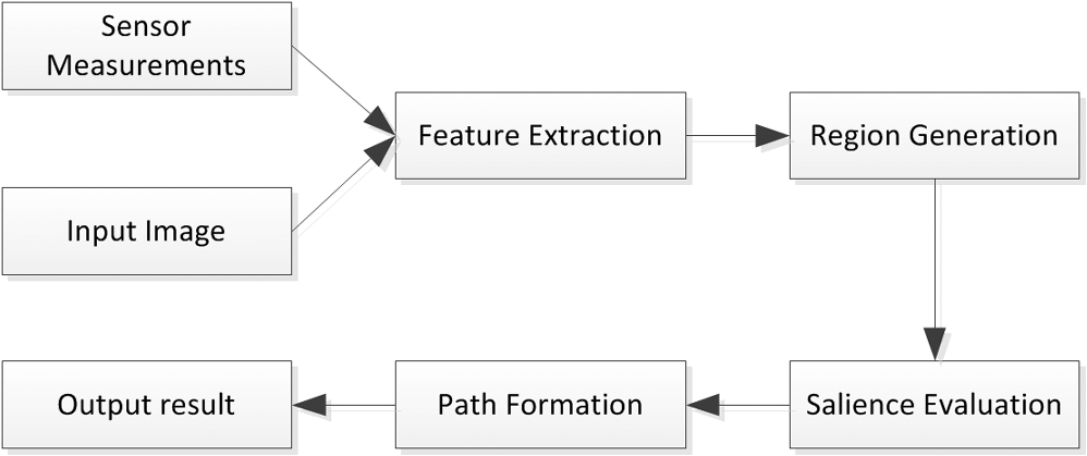

4. Results and Discussions

In Sec. 4.1, we demonstrate the superior performance of our salience model qualitatively by comparing it with two classic salience models, Itti’s model⁴ and Cheng’s model.²²^,²³ In Sec. 4.2, we show how the proposed algorithm proceeds to form the search path. During this procedure, we also illustrate that the search regions of objects can be computed quantitatively and the target can be judged whether it is salience or not.

4.1.

Saliency-Based Scene Analysis

In this section, we compare our salience model to Itti’s model and Cheng’s model for the aim of scene analysis. Itti’s model is based on local contrast with the objective to calculate the salience measure of image pixels or patches. Cheng’s model is based on global contrast with the objective to segment the salient object from the image. Although Itti’s model⁴ was published early, this model is still competitive with current state-of-the-art methods.⁵ Cheng’s model,²² published more recently,²³ proves that it outperforms other methods of the same type.

All the image patches of this experiment are acquired from Afﬁne Covariant Features Database.²⁴ The feature is constructed with the values inside a $5 \times 5$ rectangle centered at the location of the local maximum response of difference of Gaussian. We compute the salience measurements of the image patches for the three methods. The results are shown in Fig. 3, in which the higher level of saliency, the brighter the objects are in the image and the more discriminative power they have.

Fig. 3

The comparison of salience models: (a) original image patch, (b) Itti’s saliency model and (c) our saliency model, and (d) Cheng’s model. The higher level of saliency, the brighter the objects are and the more discriminative power they have.

In the scene that contains similar objects, the feature of these objects appears more frequent than that in the scene that only contains unique objects. As a result, the term $\max_{O_{j} \in Ω, O_{j} \neq O_{k}} P (f | O_{j}, I)$ is greater for the scene that contains similar objects than that for the scene that only contains unique objects. For the first row of Fig. 3, because of the existence of windows with similar appearance, our model gives a lower level of saliency than Itti’s. This result is intuitive because this image patch can hardly be used for visual search. For the second row, our model gives a higher level of saliency for the image patch because this patch contains the unique object like the tower. For Cheng’s model, it outputs a different kind of result because a different mechanism, global contrast, is adopted. For the first row, Cheng’s model captures two windows successfully. But for the second row, this model fails. According to the results, our salience model can provide more valuable evidence for visual search in these scenes.

4.2.

Visual Search

In this section, we leverage the real environment to test the validity of our method. The images are acquired from New York University (NYU) Depth Dataset V2 Dataset.²⁵ The experiment scene is shown in Fig. 4. The size of images is $640 \times 480$ , and the depth images provide the 3-D coordinates. We utilize Harris corner as the feature to represent objects. The unit of distance is meter, and the unit of angle is degree. The coordinate of the camera is (0, 0, 0), and the pose parameter is (0, 0, 0). The target, a bottle, is indicated by a cross with coordinates ( $- 0.3128$ , 0.1873, 1.323). Because of the synchronization of RGB frames and depth frames and other measure noises, the error $E$ is derived as (0.5, 0.5, 0.5, 0.1, 0.1, 0.1).

Fig. 4

The experimental scene. The target is indicated by a cross and the search region is indicated by a rectangle.

In the first step, Harris corners of the image are extracted as features, which are presented by circles in Fig. 4. Owing to the corresponding 3-D coordinates, the search region can be obtained according to Eq. (7) and indicated by a rectangle. From the result, the target cannot be found because there are objects that have a similar appearance, whichs lead to a low level of saliency. In the next step, the search path is generated to locate the target. During this processing, we need to select the salient features and judge whether the target can be found or not.

In this experiment, the first salient feature is selected with coordinates (0.1363, 0.1131, 1.487), which is shown in Fig. 5 using circle. The critical step for generating the search path is the computation of the search region when a feature is located. When the feature at the starting point of the search path has been found, the search regions of other features are calculated by Eq. (8). When more features are found, the search regions of other features are calculated in the same way. The second feature is selected with coordinate (0.8518, $- 0.2673$ , 2.5), which is shown in Fig. 6 using circle as well. The salient objects are found preferentially, and then the target can be searched in the new search region.

Fig. 5

The intermediate generated search path. Through locating one salience object, the search region of the target decreases.

Fig. 6

The final generated search path. Through the salience objects, the target can be found in the new search region.

When two salient objects join the search path, the target can be found in the new search region. According to the algorithm proposed in our paper, a search path is generated as is shown in Fig. 6 using arrows. Quantitative results are shown in Table 1. We can see that as the number of salient objects increases, the search region of the target decreases and the target becomes easier to be found.

Table 1

Generation of search path.

Number of node	The target’s search region (width, height)	Number of bottles in the target’s search region
1	(109, 101)	5
2	(60, 43)	3
3	(29, 14)	1

In Table 2, we list the performance comparisons of the computation involved in Eqs. (7) and (8). The speed of the target search can be improved by 56.7% using the optimization method compared with the Brute Force method. The results are obtained on a PC with Intel I5 CPU and 8G RAM. Brute force is executed such that position parameters are substituted iteratively in a step size of 0.05 and pose parameters in a step size of 0.1. The unit of error is subpixel, which is the max error value in width and height. We can see that approximation, and optimization has excellent running time while keeping an acceptable error. Note that we consider that brute force has the most accurate result subjectively. If we want to improve the accuracy of brute force further, a smaller step size is needed and the running time grows exponentially. More results can be found in Fig. 7. The targets are the can, the cup, and the book. The search paths that lead to the targets are shown in the second row of Fig. 7.

Table 2

Performance comparisons of brute force, approximation, and optimization.

Performance	Brute force	Approximation	Optimization
Time (ms)	104	16	45
Error (subpixel)	0	1.6	2.8

Fig. 7

More results of search path: (a) the can, (b) the cup, and (c) the book. The first row is the search region and initial features. The second row is the search path.

5. Future Developments

This paper applies key point features for salience estimation. In the future, we will use more features such as color and texture to improve salience estimation. The known knowledge of objects is also a benefit of salience estimation as a top–down tune. We will attempt to model the prior knowledge and integrate them into our salience estimation method. In Sec. 3.2.2, a simplex method is applied to determine search regions. However, this method is time-consuming, especially when a nonlinear imaging model is used to reduce the distortion effect. As a result, we will investigate other approaches to provide a more efficient solution for real-time applications.

6. Conclusion

In this paper, we propose a target search method based on salience mechanism and imaging model. This method generates a search path in which each node is a salient object with respect to its search region. When a salient object of the search path is located, search regions of the subsequent objects will decrease. The target could be found in a region that is getting smaller. The relation between salience objects and the target is used to find the target. Through these operations, target search becomes more accurate and quicker.

We want to apply our method in a real application such as visual SLAM robot. We think that this method will reduce the cost of point matching for SLAM and other similar applications. At the same time, this method is also useful for scene modeling. We will continue to explore these applications.

Appendices

Appendix:

Power Method and H_x(ξ)

A.1.

Power Method

Power method is a numerical computation method that computes the maximum eigenvalue of a matrix. The pseudo code listed in Algorithm 2 gives an implementation of power method.

Algorithm 2

Power method max λ(M)≈xT*M*x;

x = randn (m, 1)

;

x = x / norm (x)

;

do{

x 1 = x

;

x = M * x

;

x = x / norm (x)

;

} while

{abs [norm (x) - norm (x 1)] > ϵ}

A.2.

$‖$ H_x(ξ) $‖$ and $‖$ H_x(G) $‖$

Because $ξ$ locates in the interval $G \pm E$ , we make $ξ = G + δ$ where $δ = {(δ α, δ β, δ γ, δ x, δ y, δ z)}^{T}$ . We denote extrinsic parameter matrix

M = [\begin{matrix} r_{11} & r_{12} & r_{13} & 0 \\ r_{21} & r_{22} & r_{23} & 0 \\ r_{31} & r_{32} & r_{33} & 0 \\ 0 & 0 & 0 & 1 \end{matrix}] .

We have $H_{x} = [\begin{matrix} A_{3 \times 3} & B_{3 \times 3} \\ B_{3 \times 3}^{T} & 0_{3 \times 3} \end{matrix}]$ . The element of matrix $B$ has the form $b_{i j} = T_{1} T_{2} f_{x}$ , $T_{1} \in {\frac{\partial}{\partial α}, \frac{\partial}{\partial β}, \frac{\partial}{\partial γ}}$ , $T_{2} \in {\frac{\partial}{\partial t_{x}}, \frac{\partial}{\partial t_{y}}, \frac{\partial}{\partial t_{z}}}$ . So $b_{i j}$ is a function of ${α, β, γ}$ . The element of matrix $A$ has the form $a_{i j} = T_{1} T_{1} f_{x}$ , $T_{1} \in {\frac{\partial}{\partial α}, \frac{\partial}{\partial β}, \frac{\partial}{\partial γ}}$ . So $a_{i j}$ is a function of ${α, β, γ, t_{x}, t_{y}, t_{z}}$ . When $(δ α, δ β, δ γ)$ are all small increments, we have $\sin (α + δ α) \approx \sin α$ , $\cos (α + δ α) \approx \cos α$ .

According to triangle inequality principal, we have $| ‖ H_{x} (G) ‖ - ‖ H_{x} (ξ) ‖ | \leq ‖ H_{x} (G) - H_{x} (ξ) ‖$ . From the discussion above, we have

Eq. (12)

H_{x} (G) - H_{x} (ξ) \approx [\begin{matrix} \tilde{A} & 0 \\ 0 & 0 \end{matrix}] .

∵ a_{11} = (l_{x} \frac{\partial^{2}}{\partial α^{2}} r_{11} + u_{0} \frac{\partial^{2}}{\partial α^{2}} r_{31}) (x - t_{x}) + (l_{x} \frac{\partial^{2}}{\partial α^{2}} r_{12} + u_{0} \frac{\partial^{2}}{\partial α^{2}} r_{32}) (y - t_{y}) + (l_{x} \frac{\partial^{2}}{\partial α^{2}} r_{13} + u_{0} \frac{\partial^{2}}{\partial α^{2}} r_{33}) (z - t_{z})

∴ {\tilde{a}}_{11} = a_{11} (G) - a_{11} (ξ) \approx (l_{x} \frac{\partial^{2}}{\partial α^{2}} r_{11} + u_{0} \frac{\partial^{2}}{\partial α^{2}} r_{31}) δ x + (l_{x} \frac{\partial^{2}}{\partial α^{2}} r_{12} + u_{0} \frac{\partial^{2}}{\partial α^{2}} r_{32}) δ y + (l_{x} \frac{\partial^{2}}{\partial α^{2}} r_{13} + u_{0} \frac{\partial^{2}}{\partial α^{2}} r_{33}) δ z .

{\tilde{a}}_{i j}

has the same functional form as

a_{11}

.

∵nonzero eigenvalues of matrix $M$ are equal to nonzero eigenvalues of $[\begin{matrix} M & 0 \\ 0 & 0 \end{matrix}]$

∴ λ_{\max} ({\tilde{A}}^{T} \tilde{A}) = λ_{\max} [\begin{matrix} {\tilde{A}}^{T} \tilde{A} & 0 \\ 0 & 0 \end{matrix}] = λ_{\max} ([\begin{matrix} {\tilde{A}}^{T} & 0 \\ 0 & 0 \end{matrix}] [\begin{matrix} \tilde{A} & 0 \\ 0 & 0 \end{matrix}])

∴ ‖ [\begin{matrix} \tilde{A} & 0 \\ 0 & 0 \end{matrix}] ‖ = ‖ \tilde{A} ‖

∵ ‖ \tilde{A} ‖ \leq \min \max λ^{1 / 2} [{\tilde{A}}^{T} \tilde{A}] .

We will find $δ^{*} = {[δ x^{*}, δ y^{*}, δ z^{*}]}^{T}$ that minimizes the two-norm of $A (δ)$ . As a result, we need to get $δ^{*}$ to solve

{\begin{matrix} \underset{δ}{minimize} \max λ^{1 / 2} [{\tilde{A}}^{T} (δ) \tilde{A} (δ)] \\ subject to : - E ≼ δ ≼ E \end{matrix} .

This equation can be converted into a semidefinite programing problem

Eq. (13)

{\begin{cases} minimize t \\ subject to : [\begin{matrix} t I & \tilde{A} (δ) \\ {\tilde{A}}^{T} (δ) & t I \end{matrix}] ≽ 0 \\ - E ≼ δ ≼ E \end{cases} .

The output result

t

is the value that we want to obtain.

Acknowledgments

This research was supported by the National Natural Science Foundation of China (Grant No. 61272523), the National Key Project of Science and Technology of China (Grant No. 2011ZX05039-003-4), and the Fundamental Research Funds for the Central Universities.

References

1.

F. Endres et al., “3-D mapping with an RGB-D camera,” IEEE Trans. Rob., 30 (1), 177 –187 (2014). http://dx.doi.org/10.1109/TRO.2013.2279412 ITREAE 1552-3098 Google Scholar

2.

M. J. Westoby et al., “‘Structure-from-motion’ photogrammetry: a low-cost, effective tool for geoscience applications,” Geomorphology, 179 300 –314 (2012). http://dx.doi.org/10.1016/j.geomorph.2012.08.021 Google Scholar

3.

R. Hartley and A. Zisserman, Multiple View Geometry in Computer Vision, Cambridge University Press, Cambridge, United Kingdom (2003). Google Scholar

4.

L. Itti, C. Koch and E. Niebur, “A model of saliency-based visual attention for rapid scene analysis,” IEEE Trans. Pattern Anal. Mach. Intell., 20 (11), 1254 –1259 (1998). http://dx.doi.org/10.1109/34.730558 Google Scholar

5.

S. Frintrop, T. Werner and G. M. Garcia, “Traditional saliency reloaded: a good old model in new shape,” in Proc. of the IEEE Conf. on Computer Vision and Pattern Recognition, 82 –90 (2015). Google Scholar

6.

A. Borji et al., “Salient object detection: a benchmark,” IEEE Trans. Image Process., 24 (12), 5706 –5722 (2015). http://dx.doi.org/10.1109/TIP.2015.2487833 IIPRE4 1057-7149 Google Scholar

7.

X. P. Hu, L. Dempere-Marco and Y. Guang-Zhong, “Hot spot detection based on feature space representation of visual search,” IEEE Trans. Med. Imaging, 22 (9), 1152 –1162 (2003). http://dx.doi.org/10.1109/TMI.2003.816959 Google Scholar

8.

A. M. Treisman and G. Gelade, “A feature-integration theory of attention,” Cognit. Psychol., 12 (1), 97 –136 (1980). http://dx.doi.org/10.1016/0010-0285(80)90005-5 CGPSBQ 0010-0285 Google Scholar

9.

J. M. Wolfe, “Visual search,” Attention, 13 –73 University College London Press, London, United Kingdom (1998). Google Scholar

10.

N. Bruce, J. Tsotsos, “Saliency based on information maximization,” in Advances in Neural Information Processing Systems, 155 –162 (2005). Google Scholar

11.

X. Hou, L. Zhang, “Dynamic visual attention: searching for coding length increments,” in Advances in Neural Information Processing Systems, 681 –688 (2009). Google Scholar

12.

Y. Li et al., “Visual saliency based on conditional entropy,” in Computer Vision–ACCV, 246 –257 (2009). Google Scholar

13.

N. J. Butko and J. R. Movellan, “Infomax control of eye movements,” IEEE Trans. Auton. Ment. Dev., 2 (2), 91 –107 (2010). http://dx.doi.org/10.1109/TAMD.2010.2051029 Google Scholar

14.

D. S. Gao, S. Han and N. Vasconcelos, “Discriminant saliency, the detection of suspicious coincidences, and applications to visual recognition,” IEEE Trans. Pattern Anal. Mach. Intell., 31 (6), 989 –1005 (2009). http://dx.doi.org/10.1109/TPAMI.2009.27 ITPIDJ 0162-8828 Google Scholar

15.

L. Zhang et al., “SUN: a Bayesian framework for saliency using natural statistics,” J. Vision, 8 (7), 32 –32 (2008). http://dx.doi.org/10.1167/8.7.32 1534-7362 Google Scholar

16.

J. Harel, C. Koch, P. Perona, “Graph-based visual saliency,” in Advances in Neural Information Processing Systems, 545 –552 (2006). Google Scholar

17.

S. Chikkerur et al., “What and where: a Bayesian inference theory of attention,” Vision Res., 50 (22), 2233 –2247 (2010). http://dx.doi.org/10.1016/j.visres.2010.05.013 VISRAM 0042-6989 Google Scholar

18.

Z. Y. Zhang, “A flexible new technique for camera calibration,” IEEE Trans. Pattern Anal. Mach. Intell., 22 (11), 1330 –1334 (2000). http://dx.doi.org/10.1109/34.888718 ITPIDJ 0162-8828 Google Scholar

19.

J. Kannala and S. S. Brandt, “A generic camera model and calibration method for conventional, wide-angle, and fish-eye lenses,” IEEE Trans. Pattern Anal. Mach. Intell., 28 (8), 1335 –1340 (2006). http://dx.doi.org/10.1109/TPAMI.2006.153 ITPIDJ 0162-8828 Google Scholar

20.

Z. Xiang, X. Dai and X. Gong, “Noncentral catadioptric camera calibration using a generalized unified model,” Opt. Lett., 38 (9), 1367 –1369 (2013). http://dx.doi.org/10.1364/OL.38.001367 OPLEDP 0146-9592 Google Scholar

21.

O. Christensen and K. L. Christensen, Approximation Theory: From Taylor Polynomials to Wavelets, Springer Science & Business Media, Berlin, Germany (2004). Google Scholar

22.

M. M. Cheng et al., “Global contrast based salient region detection,” in IEEE Conf. on Computer Vision and Pattern Recognition, 409 –416 (2011). http://dx.doi.org/10.1109/CVPR.2011.5995344 Google Scholar

23.

M. M. Cheng et al., “Global contrast based salient region detection,” IEEE Trans. Pattern Anal. Mach. Intell., 37 (3), 569 –582 (2015). http://dx.doi.org/10.1109/TPAMI.2014.2345401 ITPIDJ 0162-8828 Google Scholar

24.

K. Mikolajczyk et al., “Affine covariant features,” (2015) http://www.robots.ox.ac.uk/~vgg/research/affine/index.html November ). 2015). Google Scholar

25.

N. Silberman et al., “NYU depth dataset V2,” (2012) http://cs.nyu.edu/~silberman/datasets/nyu_depth_v2.html November 2015). Google Scholar

Biography

Qi Wang received his BE and ME degrees in computer science from the Dalian University of Technology in 2009 and 2012, respectively. He is a PhD student at Dalian University of Technology. His current research interests include stereo vision, camera imaging, and image processing.

Xiaopeng Hu received his ME degree in computer science from the University of Science and Technology of China and his PhD from the Imperial College London, United Kingdom. He is a professor at Dalian University of Technology. He has participated in many projects as a leader. His current research interests include machine vision, wireless communication, and 3-D reconstruction.

CC BY: © The Authors. Published by SPIE under a Creative Commons Attribution 4.0 Unported License. Distribution or reproduction of this work in whole or in part requires full attribution of the original publication, including its DOI.

Citation Download Citation

Qi Wang and Xiaopeng Hu "Scene analysis for effective visual search in rough three-dimensional-modeling scenes," Journal of Electronic Imaging 25(6), 061622 (20 December 2016). https://doi.org/10.1117/1.JEI.25.6.061622

Received: 4 April 2016; Accepted: 21 November 2016; Published: 20 December 2016

Access the abstract

JOURNAL ARTICLE
9 PAGES

DOWNLOAD PAPER SAVE TO MY LIBRARY

GET CITATION

CITATIONS

Cited by 2 scholarly publications.

Explore citations on Lens.org

KEYWORDS

Visualization

3D modeling

Visual analytics

Detection and tracking algorithms

Visual process modeling

Cameras

RGB color model

1.

Introduction

Fig. 1

2.

Related Works

3.

Method Formulation

3.1.

Region-Based Salience Analysis

Definition 1.

Eq. (1)

Eq. (2)

Definition 2.

Proposition 1.

Eq. (3)

3.2.

Search Region

3.2.1.

Pinhole camera model

Eq. (4)

Eq. (5)

Eq. (6)

3.2.2.

Search region

Eq. (7)

Eq. (8)

Eq. (9)

3.2.3.

Remainder analysis

Eq. (10)

Eq. (11)

3.3.

Algorithm for Search Path

Algorithm 1

Fig. 2

4.

Results and Discussions

4.1.

Saliency-Based Scene Analysis

Fig. 3

4.2.

Visual Search

Fig. 4

Fig. 5

Fig. 6

Table 1

Table 2

Fig. 7

5.

Future Developments

6.

Conclusion

Appendices

Appendix:

Power Method and Hx(ξ)

A.1.

Power Method

Algorithm 2

A.2.

‖Hx(ξ)‖ and ‖Hx(G)‖

Eq. (12)

Eq. (13)

Acknowledgments

References

Biography

Show All Keywords

Keywords/Phrases

Search In:

Publication Years

Power Method and H_x(ξ)

$‖$ H_x(ξ) $‖$ and $‖$ H_x(G) $‖$