|
|
1.IntroductionSince 25 years ago, the definition of the wavelet has led to revolutionary achievements in the development of efficient encoding of piecewise regular signals. Their ability to detect singularities much more efficiently than Fourier transform1 has contributed to their remarkable success. The wavelet provides an optimal sparse approximation of a wide set of signals and digitalizes the continuous domain transform through the fast algorithmic implementation. Nevertheless, this latter fails when dealing with singularities along curves, i.e., functions, since reconstructing images with these anisotropic features could produce undesirable artifacts. A wavelet has only diagonal, vertical, and horizontal directions, and this limited directionality sensitivity leads to inaccurate results when dealing with multidimensional data. To overcome this drawback, some forms of directionalities have been introduced, such as the steerable pyramid,2 the directional filter banks (DFBs),3 and the two-dimensional (2-D) directional wavelet.4 A complexifyied version of wavelet was also proposed in Ref. 5 to tackle the directionality limitation by adding more precision to functions. In fact, complex wavelet offers shift-invariance and yields, at each scale, six directional sub-bands oriented at and , and , and (indiscriminately by ordinary wavelet). However, it was proven through several applications that these aforementioned methods cannot represent effectively the image singularities and its anisotropic features. A real transition occurred once Candès and Donoho6 introduced the second generation of curvelet (CT) in 2004. Since then, other multiscale geometric decompositions (MGD) were introduced to counteract the CT’s weakness, namely redundancy. In this work, we study some of these MGD and represent the characteristics behind their success. We are also interested in their application in the field of remote sensing (RS). This field has drawn a great interest with the development of multiple types of sensors, leading to a huge heterogeneous amount of data. To overcome the curse of dimensionality while providing a powerful tool for environment monitoring, planning, and decision-making, several techniques have been employed. Convolutional neural network or the deep learning7–9 represents a tendency in this field thanks to its ability to automatically discover relevant contextual features in image categorization problems.10 In the same context, sparse representation (SR),11–13 total variation,14,15 and machine learning16,17 techniques, to name a few, are also investigated for different purposes, such as enhancing spatial resolution, generating explanations, and extracting knowledge from the images. MGD, the scope of our paper, have been extensively used in several domains, namely pattern recognition18,19 and computer vision.20,21 Their use was also extended to the RS field, where we need to locate edges of roads, building, rivers, and forest to detect a potential change. Adding to that, MGD provide an analytical treatment of a scene by decomposing it in high frequencies and low frequencies. This essentially helps in fusing information from different sensors and in revealing hidden characteristics indiscriminately using only one sensor image. Therefore, we aim, in this work, at drawing attention to the MGD importance and contributions in the RS field. To the authors’ knowledge, several reviews were elaborated to describe MGD, but few of them focused on their particular use in RS. This paper is organized as follows: we present, in the first section, an overview of MGD. Then we describe their characteristics and how they have been used in the field of RS. We conclude this paper with a discussion and a conclusion. 2.Overview of Multiscale Geometric DecompositionsThe notion of scales was introduced before wavelet emergence to better localize objects in the image observation. Methods like windowing or scale introduction in Fourier transform,22,23 Laplacian pyramid (LP), and derivatives of Gaussian (DoG) were the cornerstones of ideas a few years later. The definition of the continuous wavelet was a kind of generalization of previous works in scale incorporation since the newborn transform has offered a localization in time and frequency. For numerical computation needs, the wavelet was discretized using multiresolution analysis (MRA). The MRA consists of projecting a signal successively onto subspaces (as increases, the approximation becomes coarser) and yielding both approximation and detail information (detail information is calculated from two successive approximations). Otherwise, MRA stipulates that any signal, in our case an image, could be constructed iteratively by exhibiting different characteristics in every scale. Figure 1 shows how smooth regions are emphasized in finest scale while contours are more likely to be salient in the coarsest ones. Taking advantage of the MRA, wavelet transform can address point-like singularities and offer less redundant information in scales, compared to LP and DoG. Besides, wavelet is characterized by being separable, which means that its 2-D function atoms could be written as the product of two other 1-D functions. Precisely, a wavelet’s atom is obtained by three tensor products 2-D wavelets as follows: where refers to spatial coordinates of a given point , refers to dyadic scalings, refers to scale, is translation factor, is 1-D orthogonal scaling (acts like low-pass filter), is wavelet function (acts like band-pass filter), and stands for the only three directions supported by wavelets (horizontal, vertical, and diagonal). Fig. 1(a) Smooth region revealed in finest scale (b) while contours/edges revealed in coarsest scale.  The MGD were introduced to further improve the aspect of directionality limitation, whether by using the wavelet itself combined with other treatments or by defining rules for wavelet functions. These methods can be divided into two different families:
The first family proposes to build an adapted structure of the data. For example, in order to locate singularities, the bandlet decomposes the image using wavelets combined with dyadic decompositions. Each square of the resulted segmentation contains one direction, i.e., a unique piecewise singularity. However, the second family tries to ameliorate wavelet by defining additive mathematical rules on the wavelet functions. This brings more accuracy to detect image content. A debate was settled on the strength of those families and their abilities in image understanding: smooth regions, contours, and texture. According to Ref. 24, the best representation is left an open question since it is data dependent. In this section, we represent some of the MGD and describe their main characteristics and differences. Particularly, in this paper, we are interested in some MGD that are applied in the RS field. Figure 2 illustrates a map of MGD elaborated based on Ref. 24. In fact, we have written the names of methods that will be discussed in bold, so that the reader can have a clear vision of what is treated in the coming sub/sections. 2.1.Curvelet TransformThe first generation of CT was proposed by Donoho and Duncan.25 By that definition, this transform extended the ridgelets (built on the ground of 1-D wavelets to detect segment singularity)26 to switch from a global scale analysis to fine scale analysis. The idea was to decompose the image into a set of subimages and perform ridgelet transform on each one of them. This CT transform has not shown great results because of the failure of ridgelets in diagnosing the edges. The second generation of CT is then proposed and was less redundant and faster compared to its first generation.27 Given a function , the coefficients of the continuous CT transform are defined by Eq. (1): where is a CT atom, at scale , the angle of the orientation , and position . In the frequency domain, CT coefficients are represented at discrete intervals formed by sampling the continuous curvelet transform at dyadic intervals , , in an equispaced rotated anisotropic grid, as shown in Fig. 3.Fig. 3CT frequency space tiling: to get a discrete representation, the rotated tiling is transformed into squared tiling. (a) Radial tiling, (b) angular tiling, and (c) the resulting frequency tiling of CT. 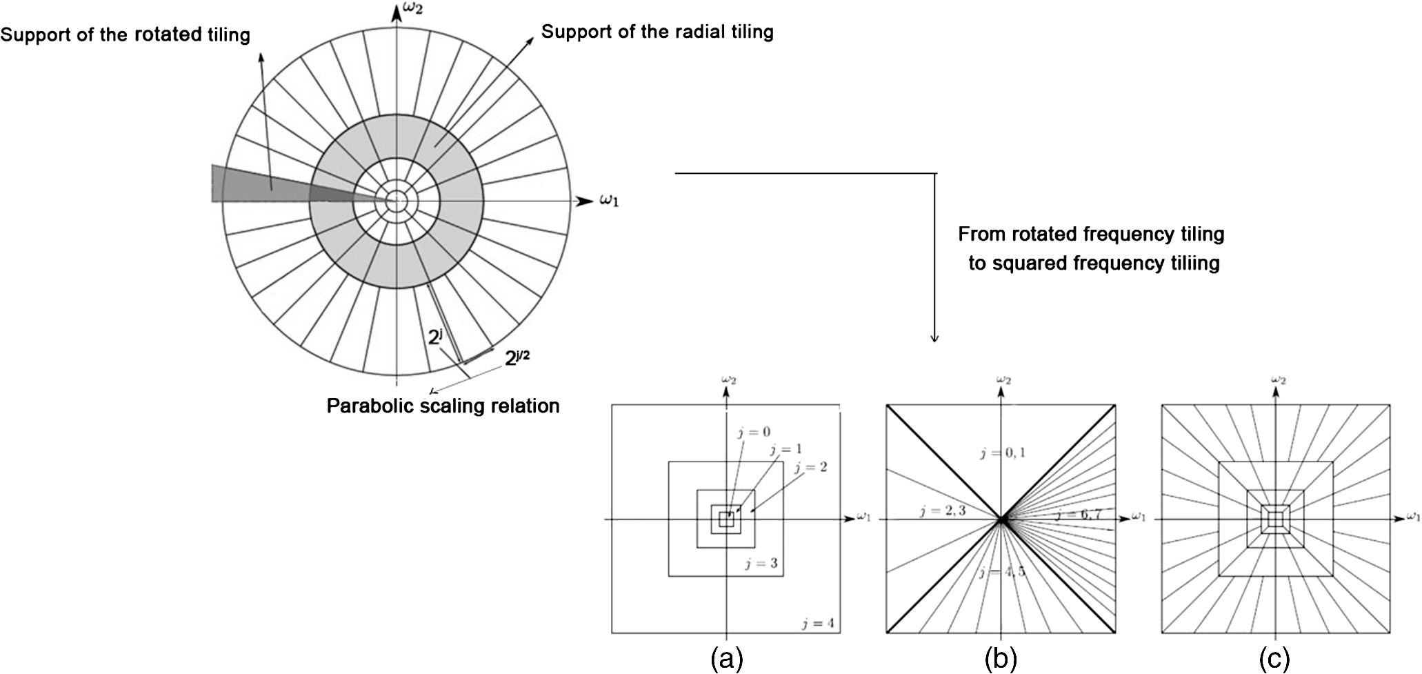 CT’s atoms are defined by a combination of a translation and a rotation of an angle of an atom : The rotation with an angle is defined as in Eq. (3):The atom of CT is defined in the frequency domain by the mean of its Fourier transform , which is written in polar coordinates as follows: where is the radial window and is the angular window at a given scale .To discretize the CT, the authors of this transform propose to switch from rotated tiling to angular tiling and from concentric circles to concentric squares, as illustrated in Fig. 3. 2.2.Contourlet TransformContourlet is considered as the extension of Candes and Donoho’s work to improve the isotropic criterion of wavelet representation.28 This transform aims at obtaining the same frequency space tiling as the CT, without the need to move from continuous to discrete domain. To do so, the authors propose a nonseparable decomposition scheme by applying a DFB, combined with LP [as shown in Fig. 4(a)] and they also propose to decrease the high redundancy information in its sub-bands. Fig. 4(a) Contourlet filter bank, the first treatment is to decompose image in multiscale sub-bands coefficients due to LP. Second, a directional decomposition filter will be applied on these coefficients. (b) Contourlet frequency space tiling.28  The DFB is designed to capture anisotropic features in the high frequencies of the image by allowing different numbers of direction at each scale while the low frequencies are processed by LP. In fact, as presented in Ref. 28, LP is defined based on orthogonal filters and downsampling by 2 in each iteration, similar to wavelet. The low-pass synthesis filter G, used for LP processing, defines a unique scaling function , that satisfies Eq. (5): where is the bandpass number, is the coordinates of a given point, and is a member of the family , which is an orthonormal basis for an approximation subspace at the scale . is a sequence of multiresolution nested subspaces.Otherwise, the DFB offers localization and directionality properties due to the family, defined in Eq. (6): which are obtained by translating the impulse responses of the equivalent synthesis filters over the sampling lattices by as follows: where corresponds to the mostly horizontal and mostly vertical sets of directions, respectively, and refers to level tree-structured DFB, which yields real wedge-shaped frequency bands (; real wedge frequency bands). The frequency tiling of this transform is shown in Fig. 4(b). The contourlet has preserved and improved the characteristics of CT. Besides, better than wavelet, the contourlet can represent edges and singularities along curves. However, the latter transform suffers from pseudo-Gibbs effect due to downsampling and upsampling. To overcome its weakness, a modified version, built on the ground of contourlet conception, was designed. The nonsubsampled contourlet transform (NSCT)29 discards the sampling step and is characterized by being shift-invariant and by preserving multiresolution criteria.2.3.Shearlet TransformShearlets30 provide a rich mathematical structure and are optimally sparse in representing the edges within an image thanks to the fact that they form a tight Parseval frame at various scales and directions. They are distinguished from CTs by being directly constructed in discrete domain, which gives them the ability to provide a more efficient multiresolution representation of the geometry.31 Besides, shearlet outperforms contourlet by substituting the directional filter with shear filter, which helps in breaking the limitation of directionalities. In the continuous domain, in dimension 2, a shearlet represents an affine system with composite dilations in Eq. (7): where is a shearlet atom, refers to the scale, refers to the shear direction, and to the translation parameter, where is the anisotropic dilation matrix (controls the support of the shearlet function) and is the shear matrix (controls the orientation). As is presented in Ref. 32, the discrete collection of shearlet transform could be defined by two window functions localized on a pair of trapezoids, as illustrated in Fig. 5(a).Fig. 5The structure of the frequency tiling by the shearlet: (a) the tiling of the frequency plane induced by the shearlets. (b) The size of the frequency support of a shearlets. (c) Shearlets conception using filters: LP combined with directional filter (shear filter).33  In fact, for a given point in the frequency domain , , and , let and where and are the mathematical definitions of vertical and horizontal cones, respectively, is a function satisfying properties in Ref. 32, and and are, respectively, truncated vertical and horizontal cones. The authors of this transform have also proposed a fast algorithmic implementation and a filter bank architecture which is similar to the one of contourlet transform as shown in Fig. 5(c)].2.4.Wedgelet TransformWedgelet is proposed by Donoho et al.34 This transform decomposes the image iteratively into piecewise constant functions (class of horizon functions). The first step consists of a dyadic recursive decomposition. In each quadtree leaf, wedgelet will search for an “edgel” in order to forward the leaf dyadic decomposition. Figure 6(a) represents a wedgelet decomposition of “cameraman” image and its dyadic decomposition. Fig. 6(a) The wedgelet segmentation process. (b) (i) Decomposition based on piecewise constant function (Wedgelet) and (ii) Decomposition based on polynomial function (Surflet).35 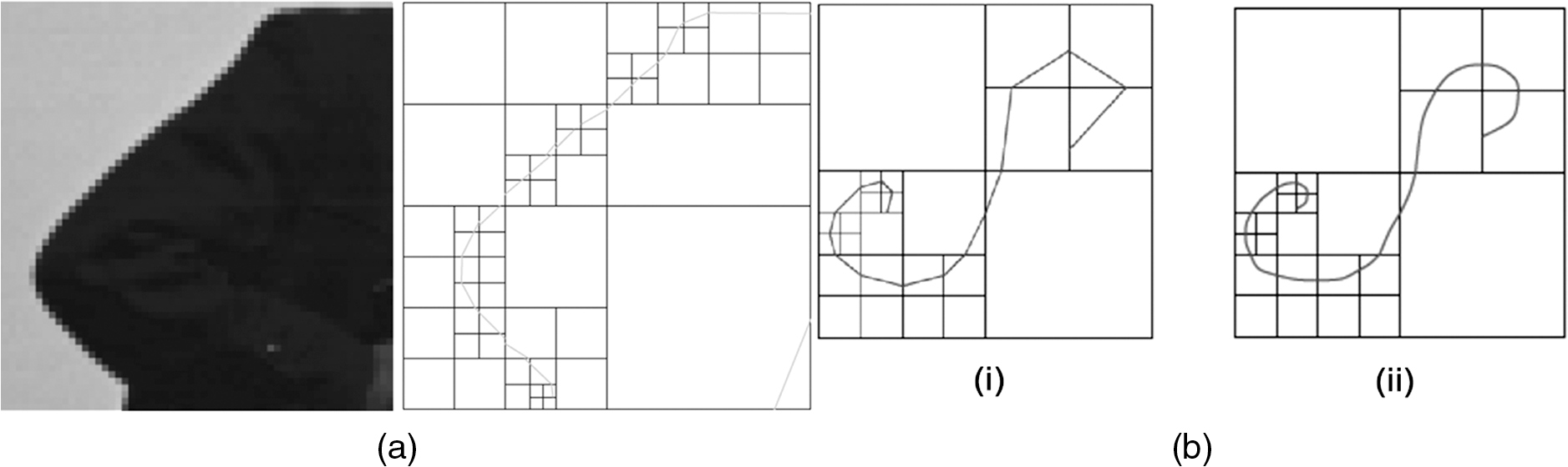 The intuitive evolution of this transform is to switch the constant horizon functions by polynomial functions in order to catch more irregular singularities. In fact, this was proposed with the surflet.36 Figure 6(b) illustrates how the dyadic decomposition is influenced when polynomial functions are used instead of piecewise constant functions. 2.5.Bandlet TransformThe first generation of the Bandlet transform was proposed by Le Pennec and Mallat.37 The main idea was to explore the wavelet transform and overcome its failure in detecting anisotropic regularities, such as curvatures. According to Ref. 37, Bandlet first performs the grassfire algorithm38 to detect edge regions and then they perform a deformation to let it fit wavelet orientations (horizontal, vertical, or diagonal). This version was redundant and failed to ensure good results, mainly in compression applications.35 Thus, the second generation of bandlet is proposed. Respecting the same adaptive approach, this version is considered as an anisotropic wavelet wrapped along the geometry flows.39 This version differs from its previous version by being based on quadtree segmentation algorithm. The idea is first to estimate irregularities in the image as a vector field, generated using the edge polynomial function estimation. A wavelet transform is then applied, after that a dyadic segmentation is performed in wavelet domain. This way, wavelet coefficients are calculated along the optimally found direction in each square. The bandlet could also be seen as a polynomial approximation in an orthogonal Alpert basis. Alpert transform is simply a wrapped wavelet transform adapted to a given irregular form, as illustrated in Fig. 7. The coefficients of the bandlet are calculated by following Eq. (8): where is an Alpert coefficient of a given point , is the wavelet mother function at , refers to the scale, and refers to the factor defining the elongation of the bandlet function. Thus, bandlet coefficients are generated by inner products of the image with bandlet function .Fig. 7(a) The original image I, (b) wavelet coefficients of I, and (c) zoom on wavelet coefficients in a square S including edge and wrapping operation of the geometric flow to align it horizontally or vertically.40 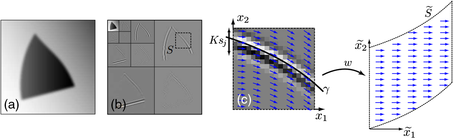 3.Characteristics of the Multiscale Geometric DecompositionsThere is no doubt that wavelet was a genuine processing tool that has led to major advances in natural image representation and understanding. Since then, many transformations have been defined to overcome the shortage of wavelet capacities by adding directions, shift invariance criteria, and so on. In Table 1, we summarized the characteristics of different transforms mentioned in this review. We have separated the MGD into two families. Their differences reside on the fact that the adaptive family constructs a special data decomposition that can fit each dataset rather than using a predefined system like the nonadaptive families. However, this adaptive form is very intensive in terms of numerical computation.1 Table 1MGD characteristics.
But, in general, all these transforms exhibit interesting parameters, which helps to bring attention to different details within an image.
Fig. 8Reconstructing images keeping only some scales. (a and b) Second and fourth scale of the CT. (c and d) Second and fourth scale of the contourlet. (e and f) Second and fourth scale of the shearlet. (g and h) Second and fourth scale of the bandlet first generation. 
The authors of bandlet have also proposed its tight frame version, which is called grouplet.44 For further details on this frame version, we refer the interested reader to Ref. 45.
4.Use of Multiscale Geometric Decompositions in Remote Sensing FieldRS images represent an efficient tool to analyze climate change and dynamics of land cover. In the last decades, a great number of new satellites has been launched, allowing a tremendous data availability with improved spatial and spectral resolutions. This has helped in enhancing our understanding and control of our surroundings. Throughout the various RS applications (image fusion, enhancement, super resolution, and so on), we are capable of monitoring the earth’s surface, predicting changes, and preventing disasters. Whereas, the management of RS images represents a challenging task. As the amount of data is incredibly growing, it is getting more complex to extract knowledge from this type of images. RS data are not only different but also have a rapid velocity and generally need several complicated corrections. That is why researchers seek new approaches to replace the traditional data processing algorithms. MGD were used in an attempt to solve some of the aforementioned problems. In fact, being able to represent the datasets in a sparse way while describing accurately, the objects in the image make the MGD an inspirational tool to be exploited in RS field. In this section, we are interested especially in the use of wavelet, CT, contourlet, shearlet, and bandlet. 4.1.ClassificationThe classification aims at recognizing the class label of a given study area with the aid of ground truth data. Conventional classification algorithms exploit essentially the spectral information of the images.48 Nevertheless, it has been proven that incorporating spatial information in the classification process, i.e., taking the contextual information into account, helps significantly in boosting the obtained accuracies. The spectral–spatial combination is possible using MGD, which not only provide a frequency representation but also help in establishing correlations between neighbors in the spatial domain. From the studied cases, we can separate the MGD use in classification in two categories:
We have studied the Ref. 49 where wavelet has been used for a feature extraction purpose. Combined with fuzzy hybridization, the wavelet coefficients are exploited for classification. The three multispectral (MS) RS images, two from Indian remote sensing and one from SPOT, are decomposed band-by-band. This technique has essentially helped in accounting for contextual information. The overall classification accuracy () using ground truth of the three images has shown that the biorthogonal wavelet exceeded the other wavelet functions. In Ref. 50, the authors proposed a CT-based approach to extract features from SAR images that can effectively identify the dynamic ice from the consolidated one. The representation of the dynamic ice contains curves in different locations with different widths and lengths and is considered larger than those of consolidated ice representation. The proposed approach consists of extracting patches from the transform domain sub-bands according to a specific size. This later increases according to the CT’s scale in order to capture more information about the curves. Once the size of patches is computed, a feature vector is calculated by Eq. (13): where is the patch with a size , denotes the mean of CT coefficients at scale , and is the total number of orientations at scale .Using SVM along with different features, the obtained experimentation results proved that the CT-based feature extraction is effective for classification since the dynamic ice area is more accurately classified. In fact, thanks to the probability density function (PDF), we can see clearly that the component representing the different types of ice could be distinguished and thus separated (Fig. 10). Fig. 10Estimated PDF for different features: (a) the PDF of SD, (b) gray-level co-occurrence matrix, and (c) CT-based method. The extracted features overlap a lot, which means they will be less effective in classification except for the PDF of CT-based method, which shows that the different types of ices could be distinguished in classification.50  Nevertheless, this quality of recognition loses its precision in CT’s finer scale. The contourlet is used in Ref. 48, where a performance comparison between wavelet and contourlet is discussed. Based on the fact that wavelet suffers from its shortage of directionality and the fact that contourlet provides directions only in high frequency coefficients, a wavelet-based contourlet transform (WBCT) is proposed and is applied on linear imaging self-scanner (LISS) II, III, and IV. Figure 11 illustrates the proposed transform. After decomposing the image using the WBCT, wavelet, and contourlet, PCA is applied to the obtained features in order to reduce their dimensionality while removing redundancy and preserving the most discriminant ones. Then a mean vector and a covariance matrix are calculated. Finally, the Gaussian kernel fuzzy C-means classifier is applied, and the obtained overall classification accuracy proves that the proposed decomposition (overall accuracy of ) is better than the wavelet-based (overall accuracy of ) and contourlet-based feature extraction methods (overall accuracy of ). As we mentioned earlier, the second category combines MGD sub-bands as features describing edges or textures, with features obtained using other methods. For example, the authors of Ref. 51 suggest to use CT jointly with morphological component analysis (MCA) and to improve RS classification using hyperspectral AVIRIS and AirSAR images. The idea is about separating a given image into two components (14): where is the smooth component, is the texture component, and is the noise. Here, the CT is used to construct a dictionary representing the smooth component and a Gabor wavelet is used to construct a dictionary representing the texture component. The authors propose to estimate the component and by solving Eq. (15) using SunSAL algorithm.52 where and are the pseudoinverse of and , respectively.This approach was extended in Ref. 53, where the authors combined several methods such as Gabor wavelet and horizontal filters to construct an MCA kernel for feature extraction. The use of such a composite kernel has given better results (overall accuracy of AVIRIS ) in characterizing image content compared to minimum noise fraction (MNF) components and helped in enhancing the characterization of the image’s content. This is explained by the fact that the proposed approach combines several methods, such as wavelet and CT. In a similar fashion, the authors of Ref. 54 proposed to combine multiple features pertaining to spectral, texture, and shape, and proposed a multiple feature combining (MFC) framework, as shown in Fig. 12. The spectral feature of a given pixel is elaborated by arranging its digital number in all of the bands. The texture feature is obtained by applying 2-D Gabor wavelet filter and the shape feature is constructed due by the pixel shape index method.55 To calculate the feature vectors using the MFC framework, a single feature-based dimensionality reduction technique is conducted in order to generate the alignment matrix. Then a Lagrangian function is calculated in order to determine the low-dimensional feature space (16): where is the alignment matrix of input samples, is the number of features (in this case 3) and is a relaxation factor with . After that, is linearized using an explicit linear projection matrix. This method outperformed several others like principal component analysis (PCA), MNF, locally linear embedding, local tangent space alignment, Laplacian eigenmaps, and achieved the optimal classification performance on HYDICE HI and ROSIS hyperspectral datasets. The criteria of assessment used in this classification were the computation of overall accuracy and the kappa index.Fig. 12Multiple features of the airborne data over the mall in Washington DC dataset. (a–c) Spectral feature images in band 36, 52, and 65. (d–f) Gabor texture feature images, with and , 3, and 5, respectively. (g–i) Shape feature images in direction 1, direction 8, and direction 16, respectively.54  4.2.Change DetectionThe detection of a change in land cover or in the Earth’s surface is considered as one of the most important applications in RS. In fact, it helps in disaster management, vegetation development, deforestation detection, and urban growth tracking. This application needs a set of multitemporal satellite images. Throughout the studied cases in this section, MGD were extensively used to ensure an accurate detection of affected regions in multitemporal images by enhancing the image’s details, especially the difference images (DIs), where noise information can easily be interfered. In Ref. 56, the contourlet is used to denoise the images of interest in order to enhance the change detection process. First, it is applied to each single temporal SAR image to preserve its features and edges. The authors also proposed to reduce speckle noise by performing hard thresholding on its high frequency sub-bands using Eq. (17): where is the variance magnitude, is the number of the decomposition coefficients at the scale , is the magnitude value of the pixel, and refers to the direction. Then the best decomposition scale is calculated by finding the minimum of the local variance of river courses magnitude. Figure 13 illustrates how the river courses are represented in SAR images and their rendering after applying contourlet.After that, markers are extracted from the contourlet domain in order to find the potential course rivers and eliminate the false alarms (content detected as river courses while it is not). After being processed, the SAR images become smoother than the ones before applying the noise and the speckle reduction. In contrast, the edges are preserved and become more visible. That is why the authors affirmed that this contourlet-based method can achieve higher accuracy of river courses detection. In Ref. 57, the CT is used jointly with MCA and is applied to a high-resolution airbone SAR image to detect changes in urban areas acquisition. The MCA decomposes the image into different components, as specified in Eq. (18): where is a transform function, is the matrix coefficients of the image in the transformed domain, and is the error (fidelity to data). In this work, the authors propose an approach using CT and wavelet-based MCA. The idea is to calculate two DIs. The first DI is obtained by computing the difference between the two SAR images. The second one is obtained by downsampling the first one. This technique is usually considered as the simplest noise suppression mechanism to use in a change detector. Then the two DIs are elaborated thanks to wavelet and CT-based MCA components as shown in Eq. (19): where the first component of is calculated using CT, is the CT function, and is the set of coefficients in CT domain. The second component of is calculated using wavelet, where is the Daubechies wavelet function and are the coefficients in wavelet domain. The corresponds to the downsampled DI by factor and it is also built using CT and wavelet-based MCA component, but this time using a different vanishing moment for the wavelet.To suppress the undesirable information, the authors applied a soft-threshold on the CT and wavelet coefficients. Then they calculated the change map, as illustrated by Eq. (20): where corresponds to a binary map obtained by Eq. (21): and corresponds to the CT component, as given in Eq. (22): The CT component, , is used to characterize the geometry of contours and edges. It also contains noise due to speckle. This noise is reduced due to the threshold , as is mentioned in Eq. (22). By calculating the change map of DI illustrated in Eq. (20), the authors aimed at obtaining a change map free of speckle noise, while conserving the contours. The experimentations show that this method can withdraw the undesirable noise without removing the cars and buildings edges. But only the geometry that has less than 8 deg of incidence angle could be maintained.In Ref. 58, the authors detected anomaly in hyperspectral images by, first, using the shearlet to decompose the images into several directional sub-bands at multiple scales. Then, in each sub-band, the background signal is reduced and the fourth-order partial differential equation is applied to brighten up the anomaly. Experimental results with HYDICE HI data show that the presented algorithm can suppress the background, detect the anomaly signal effectively, and outperform the original RX algorithm.59 Another approach is proposed using a detail-enhancing approach using NSCT Ref. 60, where the authors suggested to detect change from multitemporal optical images using a detail-enhancing approach. To do so, they studied and analyzed two change detection methods. The first61 is based on combining PCA and K-means, which was efficient in terms of computational time, but since the PCA does not consider multiscale processing, when fusing data, this has yielded false detections. The second method was proposed by Ref. 62 and introduces a multiscale framework for change detection in multitemporal SAR images. This method decomposes a DI into scales by the undecimated discrete wavelet transform (DWT). Based on this decomposition, the authors extracted a feature vector by first computing the intrascale features (sampling local neighborhood using two methods) in each sub-band in a given scale, and then by computing the interscale features, which regroup all the intrascale vectors together. The same authors improved this work in Ref. 63 by proposing the use of CT-DWT (complex wavelet) to capture further directions. The authors also used the Bayesian inference to calculate a threshold to decide whether the details to fuse correspond to changed or unchanged pixels. In Ref. 60, both works Refs. 61 and 62, were discussed. The authors estimated that the use of K-means algorithm, in Ref. 61, can stick to local optima, which can produce false detections, especially when choosing an inappropriate initial centroid. Moreover, they also affirmed that the use of wavelet, in Ref. 62, failed to characterize the geometric details of the DI efficiently. To overcome this weakness, instead of wavelet, the authors used the NSCT to decompose the DI into scales. Each scale yielded one low pass approximation sub-band and high-pass directional sub-bands . The details are extracted from directional sub-bands. The high-pass directional sub-bands serve to extract the details and are thresholded to decrease the amount of noise. The intrascale fusion is performed using max rule, as shown in Eq. (23): where is a threshold, is the scale, is a specific orientation of obtained directions from the NSCT filter bank, and corresponds to high-pass. Then the interscale fusion is applied using the max rule fusion, as well in Eq. (24):Then an enhanced DI is calculated [Eq. (25)]: where is obtained from the finest scale approximation from NSCT decomposition and is a weight to balance the emphasis between the base image and the detail image. Then the authors extract patches from , transform the patch into vector via lexicographic ordering and use PCA to produce principal components. Finally, a PCA-guided K-means64 is performed to calculate the change map. Compared to approaches based on EM, on Bayesian, on PCA, or on multiscale, the proposed approach gives better results since it conserves the geometric details due to the NSCT. The results of experimentations are illustrated in Fig. 14.Fig. 14Qualitative change detection results by using different change detection methods. (a) Ground truth change detection map created by manually analyzing the corresponding input images, (b) EM-based approach, (c) Bayesian-based approach, (d) PCA-based approach, (e) multiscale-based approach, and (f) proposed method.60  In Ref. 65, the proposed method applies wavelet on MS imagery in an anisotropic diffusion aggregation. The proposed approach is composed of three steps. We only cite, in depth, the steps where wavelet is used:
The experiments are conducted on Landsat TM and Landsat ETM+ datasets dated 1986 and 2001, respectively. The criteria of assessment used in this work are the transformed divergence measure which statistically determines the adequate wavelet levels to keep, overall accuracy and kappa. In Ref. 66, a CT-based change detection algorithm is proposed between two co-registered SAR images for natural disaster mapping. After applying the CT on the two images, the coefficients are weighted to suppress noise-like structures using the mathematical relation [Eq. (26)]: where is the amplitude found at position in the SAR image, are the sum of CT coefficients, is the number of CTs coefficients, and is a complex coefficient varying according to the image content. Finally, the change in radar amplitude is calculated by Eq. (27):4.3.FusionImage fusion represents one of the most important RS applications. It aims at combining two or more images to create another one with enhanced features. This increases the possibility of taking advantage of multisensors images and opens the door for several uses. Generally speaking, fusion can be categorized into four families based on when the fusion rule is applied: fusion at signal level, at pixel level, feature level, and decision level. The MGD belong to the feature level family. In fact, in order to conduct a fusion process with these latter decompositions, we should first convert the intrinsic image properties and get the frequency coefficients. Fusion techniques, based on MGD, suggest several injection models but tend basically to extract the spatial detail information from high spatial resolution images to inject them in the low spatial resolution ones. Compared to the largely used methods like intensity hue saturation (IHS) and PCA, MGD enhance the spatial characteristics of fused images. Thus, they look very clear, have sharp edges, and are free of spectral distortion.67 MGD-based fusion are applied abundantly in pansharpening techniques, multisensor fusion, and spatial enhancement. In Ref. 68, the authors propose a technique to fuse MS satellite images (high spectral and low spatial resolution) with a panchromatic (PAN) satellite image with low spectral and high spatial resolutions. They introduced an improved method of image fusion based on the ARSIS concept using the CT transform. The ARSIS is a French abbreviation for enhancing spatial resolution by injecting structures. CT-based image fusion has been used to merge a Landsat enhanced thematic mapper plus, PAN and MS images. Based on experimental results using indicators of bias, the CT-based method provides better visual and quantitative results for RS fusion. The indicators are
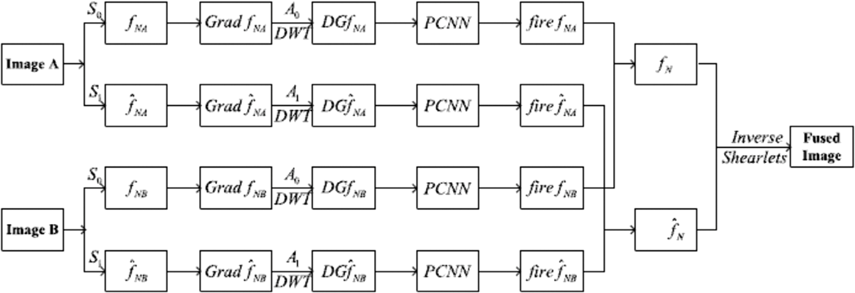
Shearlet and nonsubsampled shearlet transform (NSST) are also used in this regard. In Ref. 69, the authors propose in the first step to register two RS images. Then the shearlet transform is applied. The number of directions is set to 6 and scales to 5. The low frequency coefficients are selected based on the average rule while the high frequency coefficients are chosen using the maximum absolute value rule as mentioned in Eq. (28): where , is the absolute value of high frequency coefficients in the neighborhood of a pixel value at a location . and are equal to 3 and correspond to the size of the neighborhood window. denotes the two source images. To enhance the fusion rule for high frequencies, a decision map is produced by affecting 1 if and 0 otherwise. If some coefficients come from an image A while all its neighbors are from B, then the pixel will be extracted from B. The fusion results are illustrated in Figs. 15(a) and 15(b), which are two RS images with different band characteristics. Those two images have different physical properties of the sensor. Figures 15(c)–15(i) represent the fused images with other methods. Using shearlet, the authors assert that the obtained fusion image has clearly preserved characteristics of the surface. They found also that fusion result using contourlet has higher sharpness and entropy values than shearlet.Fig. 15Comparing shearlet fusion algorithm with other methods.69 (a) Eight-band RS image, (b) three-band RS image, (c) shearlet, (d) contourlet, (e) Haar, (f) Daubechies, (g) LP, (h) average, and (i) PCA.  In Ref. 70, the authors have used NSST.32 They have involved the SR71 paradigm in pansharpening application.72 The idea is about fusion the intensity component (I) of the MS image (the hue and saturation components are not used) with the PAN image. First, the authors decompose the images using NSST into low frequencies and high frequencies , where corresponds to scale and to direction. For the low frequency coefficients, they propose to construct vectors using patches from both and . Those vectors are represented sparsely using a learned dictionary with K-SVD73 as mentioned in Eq. (29). where is the ’th vector patch. The corresponds to the dictionary obtained by different ways: DCT, NSST and trained by K-SVD algorithm and is the sparse vector. The “absolute max” fusion rule is adopted to obtain a fused sparse coefficients (30):Then the new fused vector patch is reconstructed using the dictionary and the fused sparse coefficients are obtained as follows (31): Otherwise, the high frequency coefficients are fused according to large local energy rule. This means that the energy of each scale and direction in the shearlet transform is calculated, as mentioned in Eq. (32) and then fused: The experimental results show that the proposed method conserves better spatial and spectral information and is able to enhance the fused image better than Refs. 74 and 75. The render result is illustrated in Fig. 16. We can notice how well preserved the spatial details and color information are. Fused images have better visual accuracy compared to existing methods: AIHS,76 AWLP,75 SVT,74 and ATWT.77 Fig. 16Reference and fused images of IKONOS. (a) Original MS (R, G, and B) image; (b) original PAN image; and (c–h) the fused image using the AIHS, AWLP, SVT, ATWT, SR, and proposed method, respectively.70  The contourlets were also used78 in the same context to merge SPOT and ALSAT-2A images. The authors advanced a conception of a new fusion scheme by combining the PCA and the NSCT in order to overcome the spectral distortion caused by the PCA. The aim of this work was to find a compromise between enhancing the spatial resolution and preserving the spectral information at the same time. After decomposing the MS using PCA, a histogram matching is applied to adapt the contrast between PAN and the resulting components. Then the obtained components and PAN image are decomposed using NSCT into approximation coefficients app and details coefficients det. The fusion rules applied to this approach are represented by both Eqs. (33) and (34), where authors extract the approximation coefficients of the fused image from the PAN image and the detail coefficients from the MS image. The resulting image is obtained using Eq. (35): Then the inverse of NSCT is calculated. The fused image obtained due to the proposed method, represented edges, contours of roads and buildings, and any structure shapes on the ground, better than other method, namely intensity hue saturation (IHS), PCA-IHS, and high pass filter (HPF). Moreover, the proposed method conserves the spectral information as well. Compared to PCA-NSCT based method, the resulting fusion image was not blurred. Another injection model in pansharpening application is proposed in Ref. 79. Authors worked on QuickBird and IKONOS-2 imagery. The injection model is built on an adaptive cross gain, i.e., a ratio of local SD. Both images are decomposed using curvelets and then merged together by applying interband structure model. Compared to IHS, ATWT, and HPF, the proposed method exceeds them since it has the best rate according to the indicators: ERGAS, spectral angle mapper, and Q4. The resulted fused image is visually superior and succeeds in producing a tradeoff between different sensors. The authors of Ref. 80 propose an approach for multisensor image fusion, based on beyond the wavelet transform domain (CT, bandlet, contourlet, and wedgelet). The approach consisted of the following steps: first, the authors decomposed the images into coefficients using beyond wavelet transform. Second, they selected from the two images the low frequency coefficients using maximum local energy (MLE) rule. It is calculated in a local sliding window as shown in Eq. (36): where is the beyond wavelet low frequency coefficients, are the filter operators in different directions, and and , respectively, are the scale and direction of the transform. They obtain the fused high-frequency coefficients using the sum modified Laplacian (SML) method [Eq. (37)]: where is the modified Laplacian, or are the source images, and are the scale and the direction of transform, respectively, and finally, and determine size of the chosen window. and are variables and is a threshold. Finally, the fused image is obtained by performing an inverse beyond wavelet transform. Through a large number of experiments, they concluded that the fused images are best processed when using MLE-contourlet transform (the type of images was not mentioned).The use of several transforms in an approach could increase the quality of fusion. Works like Zhong et al.81 and Zhanga et al.82 combined wavelet and curvelet together, to enhance wavelets’ abilities. Neural networks have been also investigated in RS fusion. MGD were combined with this powerful tool in order to provide more directionalities. In fact, in Ref. 83, a fusion method of SAR images based on pulse couple neural network (PCNN)84 is proposed. The highlight of this algorithm is to use the global feature of source images and calculate the gradient information of them after being decomposed into several directions. Then wavelet is applied to decompose the images further while the high frequency coefficients are selected to be the input of PCNN to get a fire map. The max rule is applied to get the final fused image. The framework of the proposed method is detailed in Fig. 17. Fig. 18Bandlet cloud removal: (a) image contaminated with clouds shadow, (b) mask of the area to be reconstructed, (c) proposed method,85 and (d) method Li et al.86  PCNN was also used in Ref. 87. The idea is to use the contourlet hidden Markov tree (CHMT) model88 to describe the statistical characteristics of contourlet coefficients of RS images. Besides, PCNN is used in this work in order to select the high-frequency directional sub-bands. First, contourlet transform is performed on the registered multisource SAR images and then the contourlet coefficients are trained by expectation maximization algorithm to calculate their edge PDFs. The highest magnitude in low-frequency sub-bands is selected. The high-frequency directional coefficients are updated by multiplying it by its edge PDF. Finally, a new clarity saliency measure is defined and used to fuse the high-frequency sub-bands. This method is compared to others: wavelets hidden Markov trees + PCNN and CT + PCNN. The results show that CHMT-PCNN can capture more directional information. Moreover, it needs less training time even with images abundant in textures. The criteria of assessment used in this work were the mutual information, weighted fusion (evaluates the visual effect), edge-dependent fusion quality index proposed by Ref. 89 (describes edge information in the image), and common information (represents the gradient information) proposed in Ref. 90. 4.4.InpaintingThe inpainting technique consists of determining the missed area. Since the RS images are sensitive to weather conditions, the inpainting technique helps in correcting images corrupted by clouds. Indeed, the bandlet is used in Ref. 85 for regenerating a contaminated RS image by cloud. This technique is spatially based, which means that we rely only on the spatial correlation of the corrupted data in SPOT, Landsat, BDOrtho images. The paper presents a geometric reconstruction method based on the geometric data from outside the cloud-contaminated region to fill in the contaminated one. The idea is to detect the boundary points of the inpainting region and try to converge to singularity points according to a specific trajectory. This trajectory follows the geometric flow calculated due to bandlet transform of Eq. (38). The is the value of the nearest pixel in the border of the inpainting zone and it is calculated with respect to the direction of the bandlet geometric flow: where represents time, is the Euclidean distance between and . is the directional derivative of with respect to the geometric flow of bandlet. The proposed approach is able to perform long region connections. This is due to the fact that bandlet not only pays attention to the geometric flow of the studied region but also to the regularity in contours and edges, which enhance the quality of the constructed image. The render of these results is presented in Fig. 18.In Ref. 91, the authors suggest to conduct an inpainting procedure on QuickBird images. They propose to remove clouds first from low spatial resolution (LR) MS and high spatial resolution (HR) PAN, then to apply mask dodging to extract background image and compute a weight matrix. After that, they process the LR MS image by an adaptive PCA algorithm, where they choose the most representative components based on the CCs. The forward shearlet is then applied on the selected components and the HR PAN image. The shearlets were applied in this case, to enhance details and keep the edges’ information. The low frequencies of the new PAN are calculated due to the low frequencies of the selected components resulted from the adaptive PCA processed on LR MS. The high frequency coefficients of the new PAN are calculated by enhancing the resulted high frequency of shearlet coefficients, as exhibited in Eq. (39): where and are weight matrices. Given the and , the inverse of shearlet transform is applied and then a new pan sharpened image is obtained free of thin clouds. This approach is compared to wavelet-PCA and NSCT-PCA. The authors affirm that NSCT-PCA has better results in terms of preserving spectral properties.5.DiscussionsThe use of MGD leads to interesting results in the field of RS. We summarized the studied works in Table 2, where we present the methods, the data, and the criteria of assessment. To analyze all these studied cases, we propose to focus on three main axes: Table 2Overview of the methods, data and the criteria of assessment of the studied approaches in the field of remote sensing.
For the first axis, the images used in the analyzed cases were very diverse. But, some types of images are more likely to be treated by MGD than others due to their rich content. In fact, MGD are often exploited with high spatial resolution data images like IKONOS, Quickbird, and SAR Images,50,80,91 to name a few. Otherwise, they are infrequently used with coarse spatial resolution like MODIS images, where pixels are not pure and edges of regions are not sharp. However, SAR images are largely used because they are high spatial resolution images and are weather and illumination independent. Nevertheless, RS data, in general, need to be geometrically corrected due to sensors’ different ground displacements and need also to be denoised from different types of perturbations using tools such as total variation.15 In the second axis, we present the most used MGD in RS. For instance, we have noticed that the wavelet is still largely used, despite the fact that they failed in representing edges. This is explained by its high capability in representing textures and extracting spectral-based features. Besides, we found that although the shearlet is built to overcome the weakness of CT and contourlet, the experimentation results using contourlet, for example, outperformed, in some cases, the use of shearlets like in Ref. 91. Moreover, the bandlet was not widely used according to our search, as is the case of the other transforms, due to its high computational time and the high dimension of RS data. It was especially investigated in the context of inpainting since it can draw the geometric flow to follow, to fill in the missed area. The use of MGD in 3-D space is barely absent. This can be explained by the fact that it is difficult to acquire data with high spatial and temporal resolutions, simultaneously, as is the case for the video.43 The third axis is dedicated to treat the limits of MGD. Since MGD are redundant, it was noticed that in some works, the authors have used techniques of dimensionality reduction as in Ref. 91 to reduce the high number of extracted features. The bright side was the fact that this is done without affecting the discriminative power or yielding undesirable spectral distortions which is an important point to take into account when dealing with RS images. In fact, works like Ref. 49 are proposing a time consuming algorithm, which needs to be optimized. Another MGD limit is to find the adequate number of scales decomposition. To ensure the extraction of enough spatial resolution details, the decomposition level must not be too high. In Ref. 92, it was proven that a wide decomposition level affects the processing of high frequencies details. Thus, the resulted image will be sensitive to noise. Taking into consideration the characteristics of MGD subbands, the accuracy of the reconstructed image could be deteriorated if inefficient fusion rules are selected. In fact, we have noticed that in some works such as Miao et al.,69 fusing the low frequency of the transform domain using the average law was inefficient. This causes, as a matter of fact, a large detail loss, since the low frequency in the MGD domain contains most of the energy, resulting in decreasing the contrast of the fused image after reconstructing it with the inverse transform of the MGD.93 6.ConclusionIn this paper, a review of MGD and some of their applications in the RS field are presented. We described how they are useful to preserve object contours and edges and to extract feature content from images. Their common characteristic was to highlight directional analysis and adaptability to the geometry within the image. The resulted basis from these MGD were sometimes redundant in order to provide a robust representation of a given signal without losing the orthogonal/orthonormal basis properties. Nevertheless, researchers are interested in searching beyond orthogonal bases. Some works propose to learn them, some others suggest to design a hybrid basis, combining the learned basis with the predefined ones. Throughout the state-of-art elaborated from different applications in the RS fields, we have noticed that the MGD confirmed their success by being used in several applications, such as change detection between temporal high spatial resolution data. In addition, they were abundantly used to preserve edges of buildings, rivers, and vehicles, given that they are more likely to enhance details of contours in the image. They are applied as well to reduce noise by extracting high frequencies from the finest scales. The MGD are exploited in fusion applications, too, in order to reconcile between different types of data. Another important side of MGD, when combined with dimensionality reduction methods like PCA, is their capability to keep their discriminative power. This is an interesting point in the case of RS field, where it is crucial to find a compromise between fidelity to data, performance, and dimensionality. ReferencesG. Kutyniok and D. Labate,
“Introduction to shearlets,”
Shearlets, 1
–38 Springer(2012). Google Scholar
E. P. Simoncelli et al.,
“Shiftable multiscale transforms,”
IEEE Trans. Inf. Theory, 38
(2), 587
–607
(1992). http://dx.doi.org/10.1109/18.119725 Google Scholar
R. H. Bamberger and M. J. Smith,
“A filter bank for the directional decomposition of images: theory and design,”
IEEE Trans. Signal Process., 40
(4), 882
–893
(1992). http://dx.doi.org/10.1109/78.127960 Google Scholar
J.-P. Antoine et al.,
“Image analysis with two-dimensional continuous wavelet transform,”
Signal Process., 31
(3), 241
–272
(1993). http://dx.doi.org/10.1016/0165-1684(93)90085-O SPRODR 0165-1684 Google Scholar
N. Kingsbury,
“Complex wavelets for shift invariant analysis and filtering of signals,”
Appl. Comput. Harmonic Anal., 10
(3), 234
–253
(2001). http://dx.doi.org/10.1006/acha.2000.0343 ACOHE9 1063-5203 Google Scholar
E. J. Candès and D. L. Donoho,
“New tight frames of curvelets and optimal representations of objects with piecewise c2 singularities,”
Commun. Pure Appl. Math., 57
(2), 219
–266
(2004). http://dx.doi.org/10.1002/cpa.v57:2 CPMAMV 0010-3640 Google Scholar
A. Krizhevsky, I. Sutskever and G. E. Hinton,
“Imagenet classification with deep convolutional neural networks,”
in Advances in Neural Information Processing Systems,
1097
–1105
(2012). Google Scholar
L. Sergey et al.,
“End-to-end training of deep visuomotor policies,”
J. Mach. Learn. Res., 17
(39), 1
–40
(2016). Google Scholar
G. Masi et al.,
“Pansharpening by convolutional neural networks,”
Remote Sens., 8
(7), 594
(2016). http://dx.doi.org/10.3390/rs8070594 RSEND3 Google Scholar
E. Maggiori et al.,
“Fully convolutional neural networks for remote sensing image classification,”
5071
–5074
(2016). http://dx.doi.org/10.1109/IGARSS.2016.7730322 IGRSD2 0196-2892 Google Scholar
M. Xu et al.,
“Cloud removal based on sparse representation via multitemporal dictionary learning,”
IEEE Trans. Geosci. Remote Sens., 54
(5), 2998
–3006
(2016). http://dx.doi.org/10.1109/TGRS.2015.2509860 IGRSD2 0196-2892 Google Scholar
B. Song et al.,
“One-class classification of remote sensing images using kernel sparse representation,”
IEEE J. Sel. Top. Appl. Earth Obs. Remote Sens., 9
(4), 1613
–1623
(2016). http://dx.doi.org/10.1109/JSTARS.2015.2508285 Google Scholar
W. Wu et al.,
“A new framework for remote sensing image super-resolution: sparse representation-based method by processing dictionaries with multi-type features,”
J. Syst. Archit., 64 63
–75
(2016). http://dx.doi.org/10.1016/j.sysarc.2015.11.005 Google Scholar
L. I. Rudin, S. Osher and E. Fatemi,
“Nonlinear total variation based noise removal algorithms,”
Phys. D: Nonlinear Phenom., 60
(1), 259
–268
(1992). http://dx.doi.org/10.1016/0167-2789(92)90242-F Google Scholar
Q. Yuan, L. Zhang and H. Shen,
“Hyperspectral image denoising employing a spectral–spatial adaptive total variation model,”
IEEE Trans. Geosci. Remote Sens., 50
(10), 3660
–3677
(2012). http://dx.doi.org/10.1109/TGRS.2012.2185054 IGRSD2 0196-2892 Google Scholar
D. J. Lary et al.,
“Machine learning in geosciences and remote sensing,”
Geosci. Front., 7
(1), 3
–10
(2016). http://dx.doi.org/10.1016/j.gsf.2015.07.003 Google Scholar
M. Pesaresi, V. Syrris and A. Julea,
“Analyzing big remote sensing data via symbolic machine learning,”
in Proc. of the 2016 Conf. on Big Data from Space,
15
–17
(2016). Google Scholar
D. O. T. Bruno et al.,
“LBP operators on curvelet coefficients as an algorithm to describe texture in breast cancer tissues,”
Expert Syst. Appl., 55 329
–340
(2016). http://dx.doi.org/10.1016/j.eswa.2016.02.019 ESAPEH 0957-4174 Google Scholar
K. G. Krishnan, P. Vanathi and R. Abinaya,
“Performance analysis of texture classification techniques using shearlet transform,”
in Int. Conf. on Wireless Communications, Signal Processing and Networking,
1408
–1412
(2016). http://dx.doi.org/10.1109/WiSPNET.2016.7566368 Google Scholar
A. Uçar, Y. Demir and C. Güzeliş,
“A new facial expression recognition based on curvelet transform and online sequential extreme learning machine initialized with spherical clustering,”
Neural Comput. Appl., 27
(1), 131
–142
(2016). http://dx.doi.org/10.1007/s00521-014-1569-1 Google Scholar
J. Chaki, R. Parekh and S. Bhattacharya,
“Plant leaf recognition using ridge filter and curvelet transform with neuro-fuzzy classifier,”
in Proc. of 3rd Int. Conf. on Advanced Computing, Networking and Informatics,
37
–44
(2016). Google Scholar
J. Allen,
“Short term spectral analysis, synthesis, and modification by discrete Fourier transform,”
IEEE Trans. Acoust. Speech Signal Process., 25
(3), 235
–238
(1997). http://dx.doi.org/10.1109/TASSP.1977.1162950 IETABA 0096-3518 Google Scholar
R. Wilson, A. D. Calway and E. R. Pearson,
“A generalized wavelet transform for Fourier analysis: the multiresolution Fourier transform and its application to image and audio signal analysis,”
IEEE Trans. Inf. Theory, 38
(2), 674
–690
(1992). http://dx.doi.org/10.1109/18.119730 IETTAW 0018-9448 Google Scholar
L. Jacques et al.,
“A panorama on multiscale geometric representations, intertwining spatial, directional and frequency selectivity,”
Signal Process., 91
(12), 2699
–2730
(2011). http://dx.doi.org/10.1016/j.sigpro.2011.04.025 SPRODR 0165-1684 Google Scholar
D. L. Donoho and M. R. Duncan,
“Digital curvelet transform: strategy, implementation, and experiments,”
Proc. SPIE, 4056 12
–30
(2000). http://dx.doi.org/10.1117/12.381679 PSISDG 0277-786X Google Scholar
E. J. Candès and D. L. Donoho,
“Ridgelets: a key to higher-dimensional intermittency?,”
Philos. Trans. R. Soc. A: Math. Phys. Eng. Sci., 357
(1760), 2495
–2509
(1999). http://dx.doi.org/10.1098/rsta.1999.0444 Google Scholar
E. Candes et al.,
“Fast discrete curvelet transforms,”
Multiscale Model. Simul., 5
(3), 861
–899
(2006). http://dx.doi.org/10.1137/05064182X Google Scholar
M. N. Do and M. Vetterli,
“The contourlet transform: an efficient directional multiresolution image representation,”
IEEE Trans. Image Process., 14
(12), 2091
–2106
(2005). http://dx.doi.org/10.1109/TIP.2005.859376 Google Scholar
A. L. Da Cunha, J. Zhou and M. N. Do,
“The nonsubsampled contourlet transform: theory, design, and applications,”
IEEE Trans. Image Process., 15
(10), 3089
–3101
(2006). http://dx.doi.org/10.1109/TIP.2006.877507 Google Scholar
W.-Q. Lim,
“The discrete shearlet transform: a new directional transform and compactly supported shearlet frames,”
IEEE Trans. Image Process., 19
(5), 1166
–1180
(2010). http://dx.doi.org/10.1109/TIP.2010.2041410 Google Scholar
B. Biswas, A. Dey and K. N. Dey,
“Remote sensing image fusion using hausdorff fractal dimension in shearlet domain,”
in Int. Conf. on Advances in Computing, Communications and Informatics,
2180
–2185
(2015). http://dx.doi.org/10.1109/ICACCI.2015.7275939 Google Scholar
G. Easley, D. Labate and W.-Q. Lim,
“Sparse directional image representations using the discrete shearlet transform,”
Appl. Comput. Harmonic Anal., 25
(1), 25
–46
(2008). http://dx.doi.org/10.1016/j.acha.2007.09.003 ACOHE9 1063-5203 Google Scholar
X. Luo, Z. Zhang and X. Wu,
“A novel algorithm of remote sensing image fusion based on shift-invariant shearlet transform and regional selection,”
AEU—Int. J. Electron. Commun., 70
(2), 186
–197
(2016). http://dx.doi.org/10.1016/j.aeue.2015.11.004 Google Scholar
D. L. Donoho et al.,
“Wedgelets: nearly minimax estimation of edges,”
Ann. Stat., 27
(3), 859
–897
(1999). http://dx.doi.org/10.1214/aos/1018031261 Google Scholar
G. Lebrun,
“Ondelettes géométriques adaptatives: vers une utilisation de la distance géodésique,”
Université de Poitiers,
(2009). Google Scholar
V. Chandrasekaran et al.,
“Surflets: a sparse representation for multidimensional functions containing smooth discontinuities,”
in Proc. Int. Symp. on Information Theory,
563
(2004). http://dx.doi.org/10.1109/ISIT.2004.1365602 Google Scholar
E. Le Pennec and S. Mallat,
“Sparse geometric image representations with bandelets,”
IEEE Trans. Image Process., 14
(4), 423
–438
(2005). http://dx.doi.org/10.1109/TIP.2005.843753 Google Scholar
H. Blum,
“Biological shape and visual science (part I),”
J. Theor. Biol., 38
(2), 205
–287
(1973). http://dx.doi.org/10.1016/0022-5193(73)90175-6 JTBIAP 0022-5193 Google Scholar
A. Mosleh, N. Bouguila and A. B. Hamza,
“Image and video spatial super-resolution via bandlet-based sparsity regularization and structure tensor,”
Signal Process. Image Commun., 30 137
–146
(2015). http://dx.doi.org/10.1016/j.image.2014.10.010 SPICEF 0923-5965 Google Scholar
S. Mallat and G. Peyré,
“Orthogonal bandlet bases for geometric images approximation,”
Commun. Pure Appl. Math., 61
(9), 1173
–1212
(2008). http://dx.doi.org/10.1002/cpa.v61:9 CPMAMV 0010-3640 Google Scholar
G. Peyré and S. Mallat,
“Orthogonal bandelet bases for geometric images approximation,”
Commun. Pure Appl. Math., 61
(9), 1173
–1212
(2008). http://dx.doi.org/10.1002/cpa.v61:9 CPMAMV 0010-3640 Google Scholar
L. Dettori and L. Semler,
“A comparison of wavelet, ridgelet, and curvelet-based texture classification algorithms in computed tomography,”
Comput. Biol. Med., 37
(4), 486
–498
(2007). http://dx.doi.org/10.1016/j.compbiomed.2006.08.002 CBMDAW 0010-4825 Google Scholar
S. Dubois, R. Péteri and M. Ménard,
“Analyse de textures dynamiques par décompositions spatio-temporelles: application à l’estimation du mouvement global,”
in Conf. CORESA 2010,
XX
(2010). Google Scholar
S. Mallat,
“Geometrical grouplets,”
Appl. Comput. Harmonic Anal., 26
(2), 161
–180
(2009). http://dx.doi.org/10.1016/j.acha.2008.03.004 ACOHE9 1063-5203 Google Scholar
P. G. Casazza, G. Kutyniok and F. Philipp,
“Introduction to finite frame theory,”
Finite Frames, 1
–53 Springer(2013). Google Scholar
D. L. Donoho,
“Compressed sensing,”
IEEE Trans. Inf. Theory, 52
(4), 1289
–1306
(2006). http://dx.doi.org/10.1109/TIT.2006.871582 Google Scholar
J.-L. Starck, F. Murtagh and J. M. Fadili, Sparse Image and Signal Processing: Wavelets, Curvelets, Morphological Diversity, Cambridge University Press(2010). Google Scholar
K. Venkateswaran, N. Kasthuri and R. Alaguraja,
“Performance comparison of wavelet and contourlet frame based features for improving classification accuracy in remote sensing images,”
J. Indian Soc. Remote Sens., 43
(4), 729
–737
(2015). http://dx.doi.org/10.1007/s12524-015-0461-5 Google Scholar
B. U. Shankar, S. K. Meher and A. Ghosh,
“Wavelet-fuzzy hybridization: feature-extraction and land-cover classification of remote sensing images,”
Appl. Soft Comput., 11
(3), 2999
–3011
(2011). http://dx.doi.org/10.1016/j.asoc.2010.11.024 Google Scholar
J. Liu, K. A. Scott and P. Fieguth,
“Curvelet based feature extraction of dynamic ice from SAR imagery,”
in IEEE Int. Geoscience and Remote Sensing Symp.,
3462
–3465
(2015). http://dx.doi.org/10.1109/IGARSS.2015.7326565 Google Scholar
Z. Xue et al.,
“Spectral–spatial classification of hyperspectral data via morphological component analysis-based image separation,”
IEEE Trans. Geosci. Remote Sens., 53
(1), 70
–84
(2015). http://dx.doi.org/10.1109/TGRS.2014.2318332 Google Scholar
J. M. Bioucas-Dias and M. A. Figueiredo,
“Alternating direction algorithms for constrained sparse regression: application to hyperspectral unmixing,”
in 2nd Workshop on Hyperspectral Image and Signal Processing: Evolution in Remote Sensing,
1
–4
(2010). http://dx.doi.org/10.1109/WHISPERS.2010.5594963 Google Scholar
X. Xu, J. Li and M. Dalla Mura,
“Remote sensing image classification based on multiple morphological component analysis,”
in IEEE Int. Geoscience and Remote Sensing Symp.,
2596
–2599
(2015). http://dx.doi.org/10.1109/IGARSS.2015.7326343 Google Scholar
L. Zhang et al.,
“On combining multiple features for hyperspectral remote sensing image classification,”
IEEE Trans. Geosci. Remote Sens., 50
(3), 879
–893
(2012). http://dx.doi.org/10.1109/TGRS.2011.2162339 IGRSD2 0196-2892 Google Scholar
L. Zhang et al.,
“A pixel shape index coupled with spectral information for classification of high spatial resolution remotely sensed imagery,”
IEEE Trans. Geosci. Remote Sens., 44
(10), 2950
–2961
(2006). http://dx.doi.org/10.1109/TGRS.2006.876704 IGRSD2 0196-2892 Google Scholar
L. Zhu et al.,
“A novel change detection method based on high-resolution SAR images for river course,”
Optik—Int. J. Light Electron Opt., 126
(23), 3659
–3668
(2015). http://dx.doi.org/10.1016/j.ijleo.2015.08.224 Google Scholar
E. M. Dominguez et al.,
“High resolution airborne SAR image change detection in urban areas with slightly different acquisition geometries,”
in Int. Archives of the Photogrammetry, Remote Sensing & Spatial Information Sciences,
(2015). Google Scholar
H. Zhou et al.,
“Shearlet transform based anomaly detection for hyperspectral image,”
Proc. SPIE, 8419 84190I
(2012). http://dx.doi.org/10.1117/12.978636 PSISDG 0277-786X Google Scholar
H. Kwon and N. M. Nasrabadi,
“Kernel RX-algorithm: a nonlinear anomaly detector for hyperspectral imagery,”
IEEE Trans. Geosci. Remote Sens., 43
(2), 388
–397
(2005). http://dx.doi.org/10.1109/TGRS.2004.841487 Google Scholar
S. Li, L. Fang and H. Yin,
“Multitemporal image change detection using a detail-enhancing approach with nonsubsampled contourlet transform,”
IEEE Trans. Geosci. Remote Sens., 9
(5), 836
–840
(2012). http://dx.doi.org/10.1109/LGRS.2011.2182632 Google Scholar
T. Celik,
“Unsupervised change detection in satellite images using principal component analysis and-means clustering,”
IEEE Trans. Geosci. Remote Sens., 6
(4), 772
–776
(2009). http://dx.doi.org/10.1109/LGRS.2009.2025059 Google Scholar
T. Celik,
“Multiscale change detection in multitemporal satellite images,”
IEEE Trans. Geosci. Remote Sens., 6
(4), 820
–824
(2009). http://dx.doi.org/10.1109/LGRS.2009.2026188 Google Scholar
T. Celik,
“A Bayesian approach to unsupervised multiscale change detection in synthetic aperture radar images,”
Signal Process., 90
(5), 1471
–1485
(2010). http://dx.doi.org/10.1016/j.sigpro.2009.10.018 SPRODR 0165-1684 Google Scholar
C. Ding and X. He,
“K-means clustering via principal component analysis,”
in Proc. of the Twenty-First Int. Conf. on Machine Learning,
29
(2004). Google Scholar
Y. O. Ouma, S. Josaphat and R. Tateishi,
“Multiscale remote sensing data segmentation and post-segmentation change detection based on logical modeling: theoretical exposition and experimental results for forestland cover change analysis,”
Comput. Geosci., 34
(7), 715
–737
(2008). http://dx.doi.org/10.1016/j.cageo.2007.05.021 Google Scholar
A. Schmitt, B. Wessel and A. Roth,
“Curvelet-based change detection on SAR images for natural disaster mapping,”
Photogramm. Fernerkundung Geoinf., 2010
(6), 463
–474
(2010). http://dx.doi.org/10.1127/1432-8364/2010/0068 Google Scholar
C. Pohl and J. van Genderen,
“Structuring contemporary remote sensing image fusion,”
Int. J. Image Data Fusion, 6
(1), 3
–21
(2015). http://dx.doi.org/10.1080/19479832.2014.998727 Google Scholar
M. Choi et al.,
“Fusion of multispectral and panchromatic satellite images using the curvelet transform,”
IEEE Trans. Geosci. Remote Sens. Lett., 2
(2), 136
–140
(2005). http://dx.doi.org/10.1109/LGRS.2005.845313 Google Scholar
Q.-G. Miao et al.,
“A novel algorithm of image fusion using shearlets,”
Opt. Commun., 284
(6), 1540
–1547
(2011). http://dx.doi.org/10.1016/j.optcom.2010.11.048 OPCOB8 0030-4018 Google Scholar
A.-U. Moonon, J. Hu and S. Li,
“Remote sensing image fusion method based on nonsubsampled shearlet transform and sparse representation,”
Sens. Imaging, 16
(1), 1
–18
(2015). http://dx.doi.org/10.1007/s11220-014-0103-y Google Scholar
M. Elad and M. Aharon,
“Image denoising via sparse and redundant representations over learned dictionaries,”
IEEE Trans. Image Process., 15
(12), 3736
–3745
(2006). http://dx.doi.org/10.1109/TIP.2006.881969 Google Scholar
S. Li and B. Yang,
“A new pan-sharpening method using a compressed sensing technique,”
IEEE Trans. Geosci. Remote Sens., 49
(2), 738
–746
(2011). http://dx.doi.org/10.1109/TGRS.2010.2067219 Google Scholar
M. Aharon, M. Elad and A. Bruckstein,
“K-SVD: an algorithm for designing overcomplete dictionaries for sparse representation,”
IEEE Trans. Signal Process., 54
(11), 4311
–4322
(2006). http://dx.doi.org/10.1109/TSP.2006.881199 Google Scholar
S. Zheng et al.,
“Remote sensing image fusion using multiscale mapped LS-SVM,”
IEEE Trans. Geosci. Remote Sens., 46
(5), 1313
–1322
(2008). http://dx.doi.org/10.1109/TGRS.2007.912737 Google Scholar
X. Otazu et al.,
“Introduction of sensor spectral response into image fusion methods. application to wavelet-based methods,”
IEEE Trans. Geosci. Remote Sens., 43
(10), 2376
–2385
(2005). http://dx.doi.org/10.1109/TGRS.2005.856106 Google Scholar
S. Rahmani et al.,
“An adaptive IHS pan-sharpening method,”
IEEE Trans. Geosci. Remote Sens., 7
(4), 746
–750
(2010). http://dx.doi.org/10.1109/LGRS.2010.2046715 Google Scholar
A. Garzelli and F. Nencini,
“Pan-sharpening of very high resolution multispectral images using genetic algorithms,”
Int. J. Remote Sens., 27
(15), 3273
–3292
(2006). http://dx.doi.org/10.1080/01431160600554991 IJSEDK 0143-1161 Google Scholar
S. Ourabia and Y. Smara,
“A new pansharpening approach based on nonsubsampled contourlet transform using enhanced PCA applied to SPOT and ALSAT-2A satellite images,”
J. Indian Soc. Remote Sens., 44
(5), 665
–674
(2016). http://dx.doi.org/10.1007/s12524-016-0554-9 Google Scholar
A. Garzelli et al.,
“Multiresolution fusion of multispectral and panchromatic images through the curvelet transform,”
in Int. Geoscience and Remote Sensing Symp.,
2838
(2005). Google Scholar
H. Lu, L. Zhang and S. Serikawa,
“Maximum local energy: an effective approach for multisensor image fusion in beyond wavelet transform domain,”
Comput. Math. Appl., 64
(5), 996
–1003
(2012). http://dx.doi.org/10.1016/j.camwa.2012.03.017 Google Scholar
H. Zhong,
“Image processing of remote sensor using lifting wavelet and curvelet transform,”
Int. J. Control Autom., 9
(3), 215
–226
(2016). http://dx.doi.org/10.14257/ijca Google Scholar
X. Zhanga, P. Huang and P. Zhou,
“Data fusion of multiple polarimetric sar images based on combined curvelet and wavelet transform,”
in 1st Asian and Pacific Conf. on Synthetic Aperture Radar,
225
–228
(2007). http://dx.doi.org/10.1109/APSAR.2007.4418595 Google Scholar
S. Cheng, M. Qiguang and X. Pengfei,
“A novel algorithm of remote sensing image fusion based on Shearlets and PCNN,”
Neurocomputing, 117 47
–53
(2013). http://dx.doi.org/10.1016/j.neucom.2012.10.025 NRCGEO 0925-2312 Google Scholar
R. P. Broussard et al.,
“Physiologically motivated image fusion for object detection using a pulse coupled neural network,”
IEEE Trans. Neural Networks, 10
(3), 554
–563
(1999). http://dx.doi.org/10.1109/72.761712 ITNNEP 1045-9227 Google Scholar
A. Maalouf et al.,
“A bandelet-based inpainting technique for clouds removal from remotely sensed images,”
IEEE Trans. Geosci. Remote Sens., 47
(7), 2363
–2371
(2009). http://dx.doi.org/10.1109/TGRS.2008.2010454 Google Scholar
M. Li, S. C. Liew and L. K. Kwoh,
“Automated production of cloud-free and cloud shadow-free image mosaics from cloudy satellite imagery,”
in Proc. of the XXth ISPRS Congress,
12
–13
(2004). Google Scholar
S. Yang, M. Wang and L. Jiao,
“Contourlet hidden Markov tree and clarity-saliency driven PCNN based remote sensing images fusion,”
Applied Soft Comput., 12
(1), 228
–237
(2012). http://dx.doi.org/10.1016/j.sigpro.2009.04.027 SPRODR 0165-1684 Google Scholar
L. Jiao and Q. Sun,
“Advances and perspective on image perception and recognition in multiscale transform domains,”
Chin. J. Comput., 29
(2), 177
(2006). Google Scholar
G. Piella and H. Heijmans,
“A new quality metric for image fusion,”
in Proc. Int. Conf. on Image Processing,
III–173
(2003). http://dx.doi.org/10.1109/ICIP.2003.1247209 Google Scholar
V. Petrovic and C. Xydeas,
“Objective image fusion performance characterisation,”
in 10th IEEE Int. Conf. on Computer Vision,
1866
–1871
(2005). http://dx.doi.org/10.1109/ICCV.2005.175 Google Scholar
C. Shi et al.,
“Pan-sharpening algorithm to remove thin cloud via mask dodging and nonsampled shift-invariant shearlet transform,”
J. Appl. Remote Sens., 8
(1), 083658
(2014). http://dx.doi.org/10.1117/1.JRS.8.083658 Google Scholar
S. Li, B. Yang and J. Hu,
“Performance comparison of different multi-resolution transforms for image fusion,”
Inf. Fusion, 12
(2), 74
–84
(2011). http://dx.doi.org/10.1016/j.inffus.2010.03.002 Google Scholar
Y. Liu, S. Liu and Z. Wang,
“A general framework for image fusion based on multi-scale transform and sparse representation,”
Inf. Fusion, 24 147
–164
(2015). http://dx.doi.org/10.1016/j.inffus.2014.09.004 Google Scholar
BiographyMariem Zaouali received her engineering degree in 2013 from the National Institute of Applied Sciences and Technology (INSAT) in Tunisia. She is currently working toward her PhD within LIMTIC Laboratory at (ISI) in Tunisia. She is working on extracting different types of descriptors from remote sensing images using multiscale geometric decomposition. Sonia Bouzidi received her PhD and master’s degrees from the University Paris 7 Jussieu in France. She carried out her research at INRIA. She started as a professor-researcher in IUP of Evry University (Paris) in 2001. Since 2003, she has been a professor-researcher at INSAT (Tunisia). She is member of LIMTIC Research Laboratory at ISI. Her main activity is about remote sensing image processing. Ezzeddine Zagrouba received his HDR from FST/University Tunis ElManar and his PhD and engineering degree from the Polytechnic National Institute of Toulouse (ENSEEIHT/INPT) in France. He is a professor at the Higher Institute of Computer Science (ISI). He is a vice president of the Virtual University of Tunis and the director of LIMTIC Research Laboratory at ISI. His main activity is focused on intelligent imaging and computer vision, and he is a vice president of the research association ArtsPi. |
|||||||||||||||||||||||||||||||||||||||||||||||||||||||||||||||||||||||||||||||||||||||