2.1.

Feature Set for Median Filtering Detection

The median pixel values obtained from overlapping filter windows are related to one another as the overlapping windows share several pixels in common. According to this fact, most state-of-the-art MF detectors^2–5 for the feature vector used different lengths and the employed some methods for the extraction of the feature set. To extend the length of the feature vector to increase the classification ratio between the altered and unaltered images, the extraction time of the feature set and the training-testing time both take longer. In Ref. 5, kernel principal component analysis is used to reduce the length of the feature vector, therefore, additional computational time is required. Most MF detectors employ several conventional extraction methods that are processed in the space/frequency domain or use the statistical theory.

2.2.

Median Filter Residual Method

Kang et al.² used the 10-dimensional (10-D) feature vector, which was extracted from the AR coefficients of the difference in the images between the original and its MF image. They computed an MFR. In Ref. 2, the authors attempted to reduce interference from an image’s edge content and the block artifacts from JPEG compression. They proposed gathering detection features from the MFR.

The image between the original and its MF image is used to construct the AR model. The difference is referred to as the MFR, which is formally defined as

Subsequently, AR coefficients are computed as

Again, the AR coefficients are for the difference in images according to the following:

2.3.

Median Filtering Forensics Method

Yuan³ proposed detecting an MF by measuring the relationships among the pixels within a $3\times 3\text{pixel}$ window from an image. The author believed that in a median-filtered image, the gray level of the block center should occur more frequently in the block after MF. For this reason, the sets include features such as the distribution of the block median pixel value and the distribution of the number of distinct gray levels within a window. Moreover, the author proposed a median filter detector that collects blockwise the MFF, which is statistically based on the pixel values and their distribution on the block. A set of five features in the MFF is extracted from a $3\times 3\text{pixel}$ nonoverlapping block:

A direct combination of these feature subsets results in a 44-dimensional feature vector (note that the $h_5^{\mathrm{DBC}}$ and the $h_5^{\mathrm{DBM}}$ are equivalent)

Different features of the MFF are then combined heuristically to produce a new index $f$, and MFD is then obtained by simply thresholding $f$

3.1.

Variation of Neighboring Line Pairs

In an image $x$, the intensity gradient between the neighboring line pairs (the row and column directions) are defined as ${\mathcal{G}}^{(r)}$ and ${\mathcal{G}}^{(c)1}$, respectively, as follows:

Furthermore, the row and column differences of the Fourier transform (FT) coefficient (${\mathrm{FT}}_{\mathrm{coeff}}$) between the neighboring line pairs are defined as ${\mathcal{F}}^{(r)}$ and ${\mathcal{F}}^{(c)}$, respectively, in the same manner of Eq. (8)–(10), to as follows:

3.2.

Feature Vector Composition

The feature set for the proposed variation-based MFD method is composed of 19-dimensions (19-D). The $k$ in ${\mathcal{G}}_k$ is set to be 1 to 9, which are the nine most significant values by descending order of ${\mathcal{G}}_k$, and the $k$ in ${\mathcal{F}}_k$ is set to be 1 to 10, the 10 most significant values by descending order of ${\mathcal{F}}_k$. Both $k$s are defined as the feature vector length based the variations of $\mathcal{G}$ and $\mathcal{F}$.

The first 9-dimensional (9-D) part is related to the variation that is the differences between the intensity values between neighboring line pairs. The nature of the feature and length is similar to the MFF OBC³ according to the space domain processing. The second 10-D part is related to the variations that are the differences between the coefficient values of FT between neighboring line pairs. The nature of the feature and length is similar to the MFR AR² according to the frequency domain processing.

The proposed complete MFD technique can be summarized as follows:

4.1.

Experimental Methodology

SVM training and testing was performed by inputting the constructed 19-D feature vector to an SVM classifier for the training of the MF classification. $C$-SVM⁷ with Gaussian kernel is employed as the classifier

The experiments prepared the following image database:

This results in the image database and, where necessary, the images were converted to 8-bit grayscale images and used in the experiments.

For the effective measurement of the proposed method in the experiment, four kinds of test items, area under curve (AUC), the classification ratio, the minimal average decision error ($P_{\mathrm{e}}$), and $P_{\mathrm{TP}}$ at $P_{\mathrm{FP}}=0.01$ ($P_{\mathrm{TP}}$ and $P_{\mathrm{FP}}$ denote the true-positive and false-positive rates, respectively). Also, the classified rate of the experimental AUC results is interpreted using the traditional academic point system. The definition of AUC grade is described in Ref. 11

Subsequently, the trained classifier model is used to perform the classification on the testing set. Among the total of 16,538 images, 10,000 images are selected randomly in training, and the other 6538 images are for testing. Before an SVM classifier is trained for the MFD, it prepared the $\mathrm{MF}w$ ($w\in \{3,5,35\}$,) for the positive data, and the negative data are three groups, $\mathcal{A}$, $\mathcal{B}$, and $\mathcal{C}$, as follows:

4.2.

Experimental Results

The proposed method compared with existing works: the MFR AR² and the MFF methods.³ For the proposed method, the experiments were conducted using the MATLAB^® (R2015a) tools on PC environment (the 64-bit version of Windows 7, Intel^® core™ i7-5960X CPU @ 3.00 GHz and DDR4 32 GB memory).

The extracted feature set distribution of variety images from the proposed variation-based MF detector is shown in Fig. 1. The JPEG ($\mathrm{QF}=90$) is very similar to the original image, but the rest of the images are quite different from each other. Figures 2 and 3 show the variations of the gradient difference and the coefficient difference of the neighboring line pairs by Eqs. (10) and (13), respectively.

Fig. 1

Distribution of the features extracted from different types of sample images: the group images (a) $\mathcal{A}$, (b) $\mathcal{B}$, (c) and $\mathcal{C}$.

Fig. 2

Variations of the gradients differences.

Fig. 3

Variations of the FT coefficient differences by Eq. (13).

In Fig. 4, receiver operating characteristic (ROC) curves show each performance of $\mathrm{MF}w$ versus the test image groups $\mathcal{A}$, $\mathcal{B}$, and $\mathcal{C}$, on the MFR AR method. In this part, the MFR AR method shows the best performance of the MFD against the UP, while, the performances of the DN, JPG, and ORI are relatively lower.

Fig. 4

ROC curves of the MFR AR method. (a) MF3 versus test images of group $\mathcal{A}$, (b) MF5 versus test images of group $\mathcal{A}$, (c) MF35 versus test images of group $\mathcal{A}$, (d) MF3 versus test images of group $\mathcal{B}$, (e) MF5 versus test images of group $\mathcal{B}$, (f) MF35 versus test images of group $\mathcal{B}$, (g) MF3 versus test images of group $\mathcal{C}$, (h) MF5 versus test images of group $\mathcal{C}$, and (i) MF35 versus test images of group $\mathcal{C}$.

In Fig. 5, ROC curves show each performance on the MFF method. In this part, the MFF method shows the best performance of the MFD in the JPEG and DN, but the performance is relatively low in UP.

Fig. 5

ROC curves of the MFF method. (a) MF3 versus test images of group $\mathcal{A}$, (b) MF5 versus test images of group $\mathcal{A}$, (c) MF35 versus test images of group $\mathcal{A}$, (d) MF3 versus test images of group $\mathcal{B}$, (e) MF5 versus test images of group $\mathcal{B}$, (f) MF35 versus test images of group $\mathcal{B}$, (g) MF3 versus test images of group $\mathcal{C}$, (h) MF5 versus test images of group $\mathcal{C}$, and (i) MF35 versus test images of group 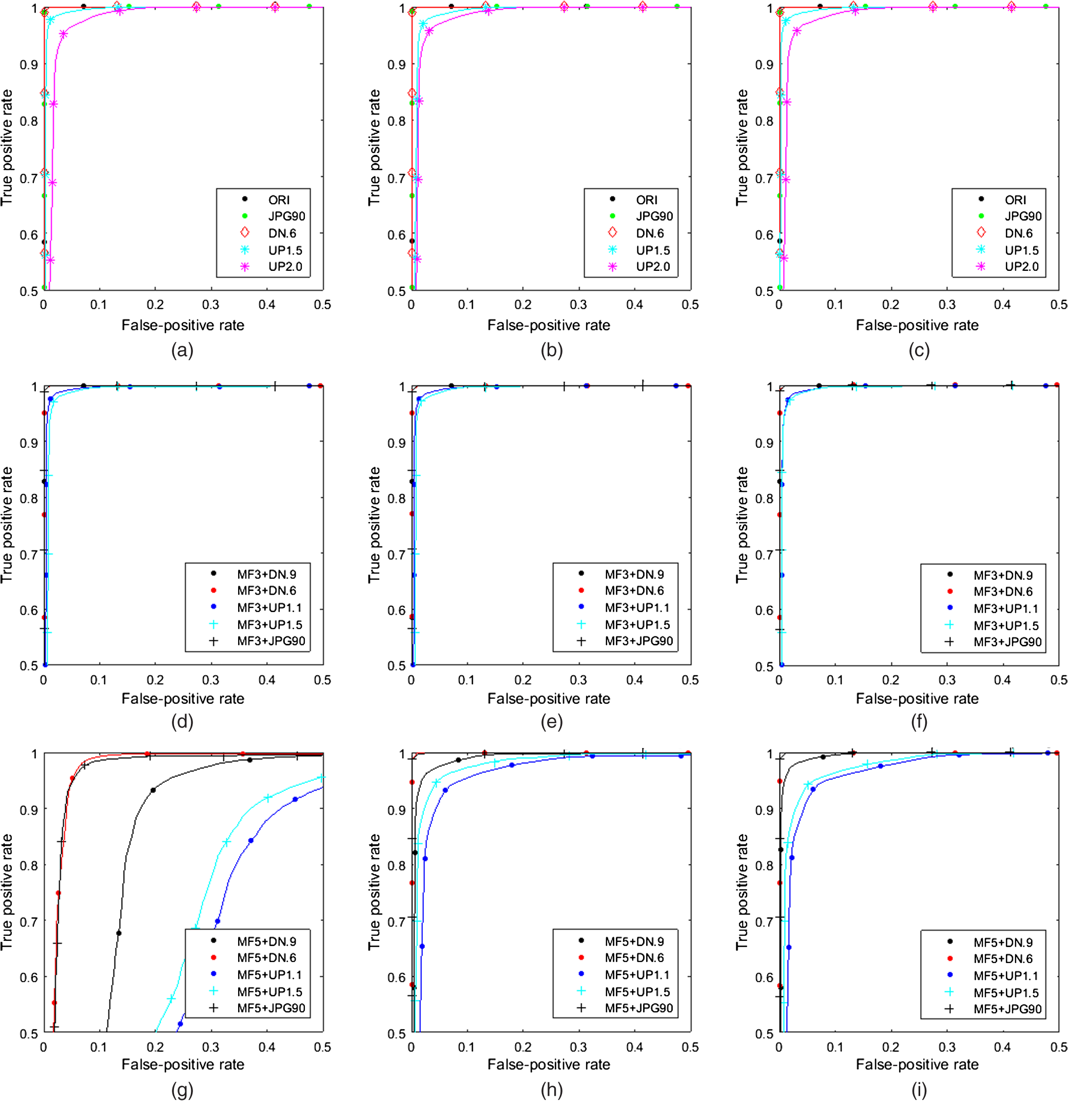$\mathcal{C}$.

In Fig. 6, the proposed method exhibits excellent performance on all $\mathrm{MF}w$ versus almost test image groups, except for MF5 versus ORI. It conducted performance evaluation and theoretical analysis for the MFD in the various altered image types.

Fig. 6

ROC curves of the proposed variation-based MFD method. (a) MF3 versus test images of group $\mathcal{A}$, (b) MF5 versus test images of group $\mathcal{A}$, (c) MF35 versus test images of group $\mathcal{A}$, (d) MF3 versus test images of group $\mathcal{B}$, (e) MF5 versus test images of group $\mathcal{B}$, (f) MF35 versus test images of group $\mathcal{B}$, (g) MF3 versus test images of group $\mathcal{C}$, (h) MF5 versus test images of group $\mathcal{C}$, and (i) MF35 versus test images of group 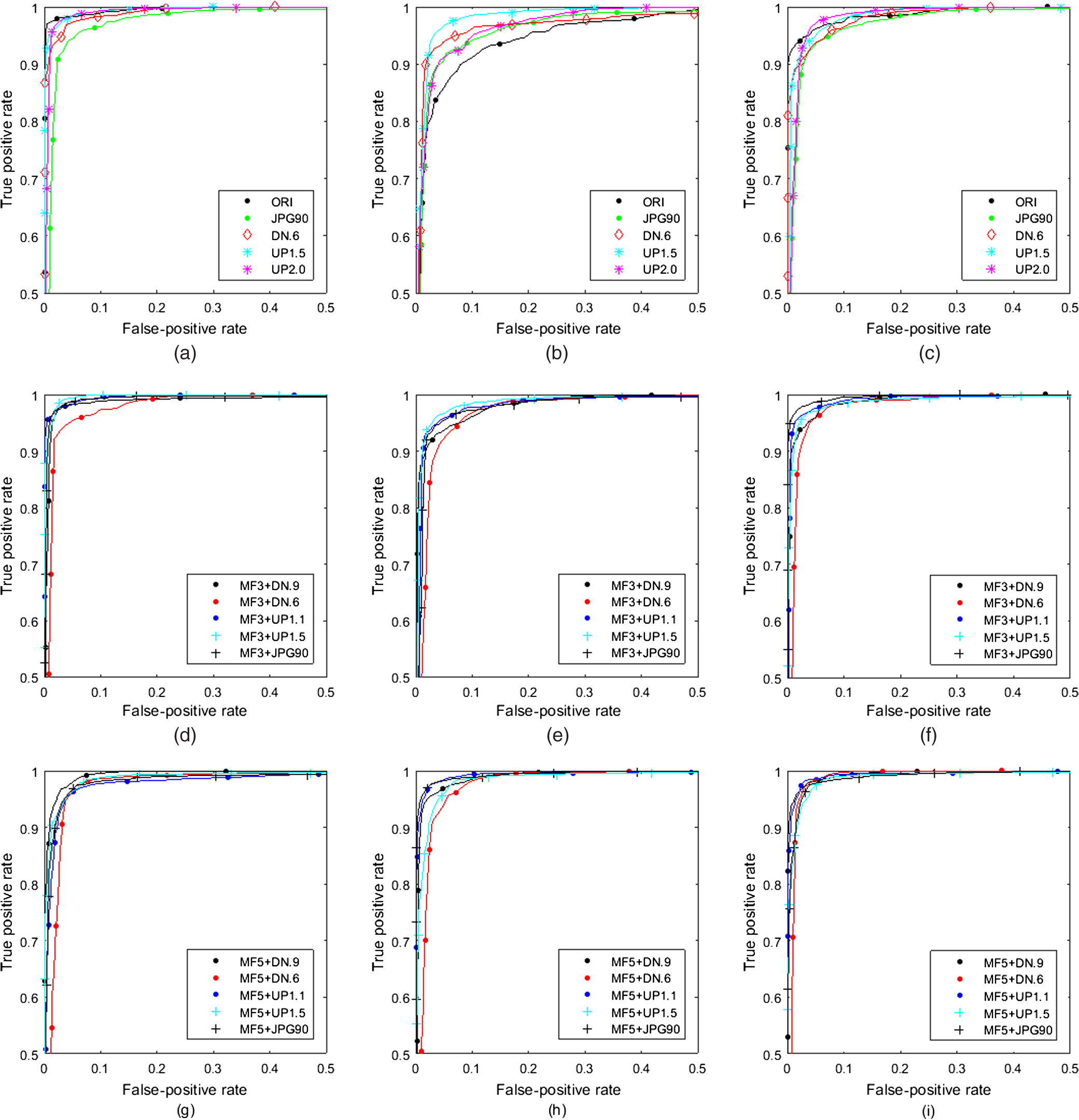$\mathcal{C}$.

Table 1 shows experimental results of $\mathrm{MF}w$ and the test image groups $\mathcal{A}$, $\mathcal{B}$, and $\mathcal{C}$, which presented as (a), (b), and (c), respectively. In this table, there are four kinds of test terms: AUC, the classification ratio, $P_{\mathrm{e}}$, and $P_{\mathrm{TP}}$ at $P_{\mathrm{FP}}=0.01$. As a result, the AUC and the classification ratio are both above 0.9. $P_{\mathrm{e}}$ ranges from 0.003 to 0.027, and $P_{\mathrm{TP}}$ at $P_{\mathrm{FP}}=0.01$ ranges from 0.965 to 0.996.

Table 1

Performance comparison between the MFR AR, MFF, and the proposed method. (The best result for each training–testing pair is displayed in bold type as a whole.) No. (experimental result item) 1: AUC, 2: classification ratio, 3: Pe, 4: PTP at PFP=0.01.

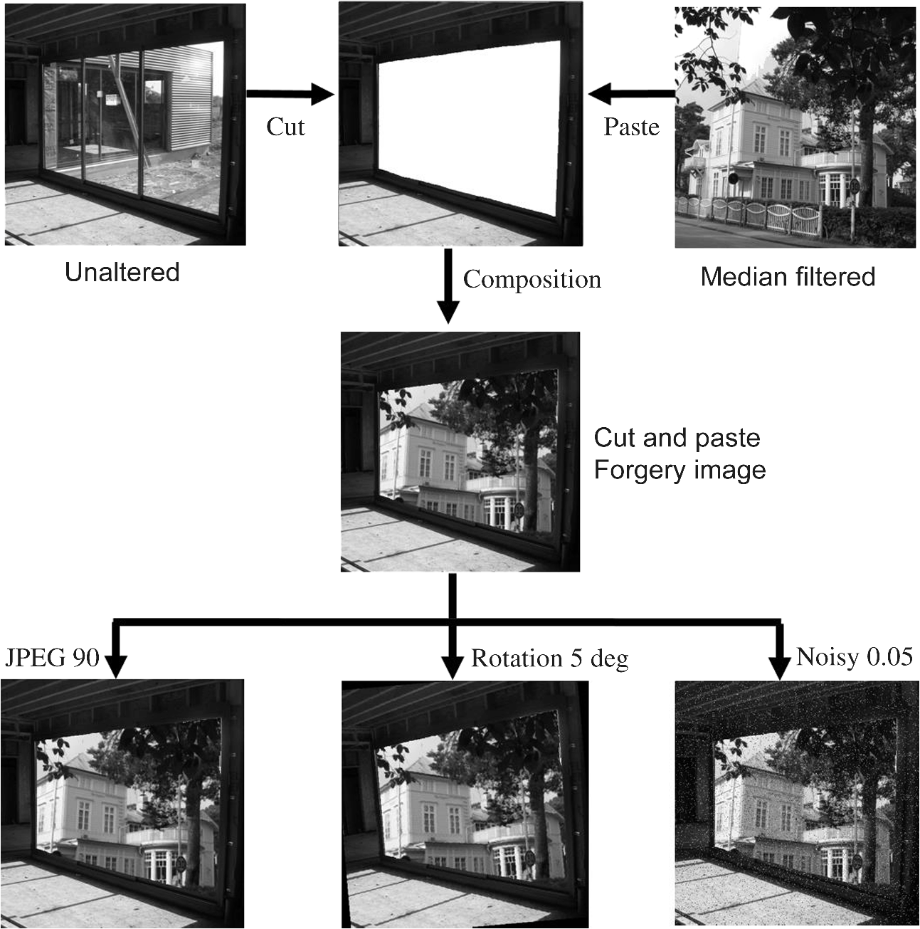
Moreover, the ROC curves of the proposed method for the many types of the test image are relatively closer to each other, which indicates the more consistent classification performance of the proposed method. Overall, the performance is excellent at unaltered (original), JPEG ($\mathrm{QF}=90$) compression, downscaling (0.6), and upscaling (1.5 and 2.0) images on the MF3, the MF5, and the MF35 detections. However, in the proposed variation-based MFD methods, despite the 19-D short length of the feature vector, the performance results of the AUCs approached 1. Thus, it is confirmed that the grade evaluation of the proposed algorithm is rated as “Excellent (A).” [The classified rate of the experimental AUC results is interpreted using the traditional academic point system¹¹ (June 2016).] In this evaluation, it uses the terms of general interpretation AUC for each training–testing pair.

Subsequently, the testing of the MF to detect low-resolution images will be examined. A small image window size is a requirement for detecting forgeries in a median-filtered image or modified JPEG pre- or/and postcompression. An example of a cut-and-paste forgery image is shown in Fig. 7. An unaltered image (window) is cut, and a median-filtered image (house) is pasted onto the cut area (white region) of the unaltered image (those unaltered images come from the BOWS2 database), forming a composite image, which was then JPEG postcompressed using a quality factor of 90, rotated counterclockwise by 5 deg and added salt and pepper noise by 0.05 density. Figures 8Fig. 9–10 show the detection blocks of MF with the MFR AR, the MFF, and the proposed method, respectively. The detected blocks that are median-filtered (the true positives) are marked in red, and the remaining blocks are marked in blue (the false alarms). (The color version of the paper is available online.) In Figs. 8Fig. 9–10, the left column (a, c, e, and g) is examined in a $32\times 32$ block size, and the right column (b, d, f, and h) is examined in a $64\times 64$ block size. The first row (a and b) shows the detection results in MF3 versus unaltered images, the second row (c and d) shows the detection results in MF3 + JPG90 versus JPG90 images, the third row (e and f) shows the detection results in MF3 versus unaltered to rotated images, and the last row (g and h) shows the detection results in MF3 versus unaltered to noisy images.

Fig. 7

Cut and paste forgery image example.

Fig. 8

Local MFD results using the MFR AR method.

Fig. 9

Local MFD results using the MFF method.

Fig. 10

Local MFD results using the proposed method.

In Fig. 8, the MFR AR method does not perform well for a $32\times 32$ size image, and it performs only slightly better for MF3 versus unaltered images on a $64\times 64$ size image. In Fig. 9, the MFF method performed well for MF3 versus unaltered images and rotated one for both $32\times 32$ and $64\times 64$ size images. Meanwhile, the corresponding forensic detection does not provide good results in JPEG postcompression. In Fig. 10, the MFD of the proposed method with a 19-D feature vector is supreme for MF3 versus unaltered images, under JPEG postcompression, and its rotated and noisy one for both $32\times 32$ and $64\times 64$ size images, respectively.