Image segmentation on adaptive edge-preserving smoothing

Kun He; Dan Wang; Xiuqing Zheng

doi:10.1117/1.JEI.25.5.053022

4 October 2016 Image segmentation on adaptive edge-preserving smoothing

Kun He, Dan Wang, Xiuqing Zheng

Author Affiliations +

Journal of Electronic Imaging, Vol. 25, Issue 5, 053022 (October 2016). https://doi.org/10.1117/1.JEI.25.5.053022

Abstract

Nowadays, typical active contour models are widely applied in image segmentation. However, they perform badly on real images with inhomogeneous subregions. In order to overcome the drawback, this paper proposes an edge-preserving smoothing image segmentation algorithm. At first, this paper analyzes the edge-preserving smoothing conditions for image segmentation and constructs an edge-preserving smoothing model inspired by total variation. The proposed model has the ability to smooth inhomogeneous subregions and preserve edges. Then, a kind of clustering algorithm, which reasonably trades off edge-preserving and subregion-smoothing according to the local information, is employed to learn the edge-preserving parameter adaptively. At last, according to the confidence level of segmentation subregions, this paper constructs a smoothing convergence condition to avoid oversmoothing. Experiments indicate that the proposed algorithm has superior performance in precision, recall, and F-measure compared with other segmentation algorithms, and it is insensitive to noise and inhomogeneous-regions.

1. Introduction

As a technology used to extract a region of interest automatically or semiautomatically, image segmentation is a key step in image analysis and understanding studies.¹ It is used for object model representation, parameter extraction, object recognition, and for video encoding of objects in MPEG4.² Until now, there have been lots of segmentation methods for all kinds of purposes, such as organ extraction in medical applications³ and object detection in the remote sensing systems.⁴ However, they are all only used for some specific purposes, and it is difficult to generalize them to any image segmentation tasks. Consequently, a uniform segmentation framework is required for researchers and developers.⁵

Generally, image segmentation is implemented based on similarity and dissimilarity among subregion features,⁶ such as color, intensity, statistical characteristics, and specific shape. However, real images contain a large amount of inhomogeneous subregions and are unavoidably affected by noise. On the one hand, inhomogeneous subregions may form weak edges or deteriorate the similarity of the subregion, i.e., intensity uniformity. On the other hand, since noise causes pseudo-edges and weakens the significant difference among subregions,⁷ the nonrobustness of the subregion characteristics is aggravated.

Active contour models for image segmentation are popular algorithms for dividing an image into foreground and background. The basic idea is a deformable curve, which conforms to various shapes of objects. Combining the piecewise smoothing with the statistical properties of the noise, Chan and Vese proposed the region-based active contour model (CV model).⁸ In this model, the object and background regions are represented as the mean of subregions respectively. Thus, it is insensitive to noise and helpful for enhancing the computational efficiency of the Mumford–Shah model.⁹

The results of segmentation using the CV model are unsatisfactory for real images. The reason is that in-homogeneity reduces significant differences of the mean of subregions. In order to improve the segmentation performance, Tsai and Yezzi proposed a piecewise smooth (PS) model¹⁰ by approximating pixels of subregion into a function. Compared to the CV model, the PS model is insensitive to inhomogeneous subregions, but it is difficult to apply it in practice due to the expensive computational cost. Therefore, Li and Kao proposed a local binary fitting model,¹¹ which employs the Gauss kernel function to approximate the neighborhood pixels of the active contour. Peng and Liu proposed an active contour model driven by normalized local image fitting energy.¹² Although the above models have strong locating capabilities, the results of segmentation rely on the assumption of approximation function and the initial curve.

In order to overcome these shortcomings, a large number of research works were investigated. To strengthen the robustness of the initial curve, Jiang and Feng proposed a segmentation model based on improved level set and region growth, which takes the statistical information of an object as seed.¹³ Based on regional-similarity and the level set, Kong and Wang proposed the segmentation model to improve the hypothesis of approximation function model.¹⁴

Although region-based active contour segmentation models are generally robust to noise, they are valid only for images with homogeneous region given the number of subregions. According to the relationship between contour and edge, Li et al. proposed an edge-based active contour segmentation model.¹⁵ Unfortunately, it is sensitive to noise and inhomogeneous subregions. To cope with this, images are often smoothed with a Gaussian filter. However, a Gaussian filter is an isotropic point diffusion that crosses the boundaries of subregions and leads to the level set curve converging at the neighbor of object contours. Furthermore, a Gaussian filter with large standard variance may seriously blur boundaries formed by weak edges. This leads to the overconvergence of curves, and conversely the curves will be premature. It is difficult to adaptively choose standard variance for different regions in an image.¹⁶ By incorporating prior object-shape information into the initial evolving curve, Yeo and Xie improved the accuracy of segmentation for specific shape regions.¹⁷

Under- and over-segmentation phenomenon exist when traditional active contour models are applied to real images due to inhomogeneous subregions and weak edges. In order to smooth the inhomogeneous subregions and preserve edges, we propose the smoothing conditions for image segmentation: (1) isotropic smoothing inside the subregions and (2) anisotropic smoothing along the edge. Unfortunately, the aforementioned conditions are incompatible. Inspired by total variation,¹⁸ we construct an edge-preserving smoothing model, which is a compromise of the above conditions. Further, due to the location of edges, a fixed edge-preserving parameter is not a reasonable trade-off between edge-preserving and subregion smoothing. It will cause blurred-edges and residual nonuniformity in the smoothing component. To solve this problem, we investigate the two-clustering algorithm of center pixel and four neighbors to adjust the edge-preserving parameter adaptively. Fixed-point iteration is employed to compute the smoothing component. While the number of iteration is high, the smoothing component converges to the mean of the image, and the difference between the feature of an object and that of the surrounding region is not significant. To avoid these, we construct a smoothing convergence condition according to the confidence level of segmentation subregions on different smoothing components. The experimental results show that this segmentation model is insensitive to noise and inhomogeneous-regions.

The outline of the paper is as follows. In the next section, two conditions on image piecewise smoothing are proposed to construct an edge-preserving smoothing model, and the clustering algorithm is employed to learn the edge-preserving parameter. In Sec. 3, a new segmentation model for the edge-preserving smoothing component is proposed. The proposed image segmentation model is implemented in Sec. 4. The experimental results are given in Sec. 5. Finally, the conclusion is given in Sec. 6.

2. Proposed Edge-Preserving Model

The active contour model for image segmentation is curve evolution implementation based on the Mumford–Shah model.⁹ It is formulated as the following minimization problem:

Eq. (1)

E (u, C) = \frac{τ}{2} \int_{Ω} {[u (x, y) - u_{0} (x, y)]}^{2} d x d y + \int_{Ω / C} {| \nabla u (x, y) |}^{2} d x d y + γ ‖ C ‖,

where

C

is the segmentation curve,

u_{0} : Ω \to [0,1]

is a given image,

u

is a piecewise smoothing component of an image

u_{0}

and contains homogeneous subregions and significant differences among subregions. The piecewise smoothing component

u

is a solution of the following problem:

Eq. (2)

\inf_{u} {E (u, C) = \frac{τ}{2} \int_{Ω} {(u - u_{0})}^{2} d x d y + \int_{Ω / C} f (| \nabla u |) d x d y} .

To analyze the diffusibility performance for the smoothing function

f (| \nabla u |)

, the function

f (| \nabla u |)

is decomposed using the local image structures, i.e., the tangent and normal directions. The diffusibility performances along the tangent and normal directions are denoted by

ρ_{T}

and

ρ_{N}

, respectively:

Eq. (3)

ρ_{T} = \frac{f^{'} (| \nabla u |)}{| \nabla u |}, ρ_{N} = f^{''} (| \nabla u |) .

2.1.

Edge-Preserving Smoothing

In order to smooth subregions and preserve edges for real images, the diffusibility performance of the function $f (| \nabla u |)$ along the tangent and normal directions should satisfy the following two conditions:

1. Inside the subregion where gradients are low, we would like to encourage smoothing along the tangent and normal directions, which makes the intensities of the subregions equal or nearly equal to constant. In other words, it is isotropic diffusion. Assume that the function is regular, this condition may be achieved by imposing:
Eq. (4)
$\lim_{| \nabla u | \to 0} ρ_{T} = \lim_{| \nabla u | \to 0} ρ_{N} = α > 0 .$
2. In an edge where the image presents a strong gradient, we prefer to diffuse along this edge and not across it. To do this, it is sufficient to annihilate, for strong gradients, the coefficient of $ρ_{N}$ and assume that the $ρ_{T}$ does not vanish:
Eq. (5)
$\lim_{| \nabla u | \to \infty} ρ_{T} = β > 0, \lim_{| \nabla u | \to \infty} ρ_{N} = 0 .$

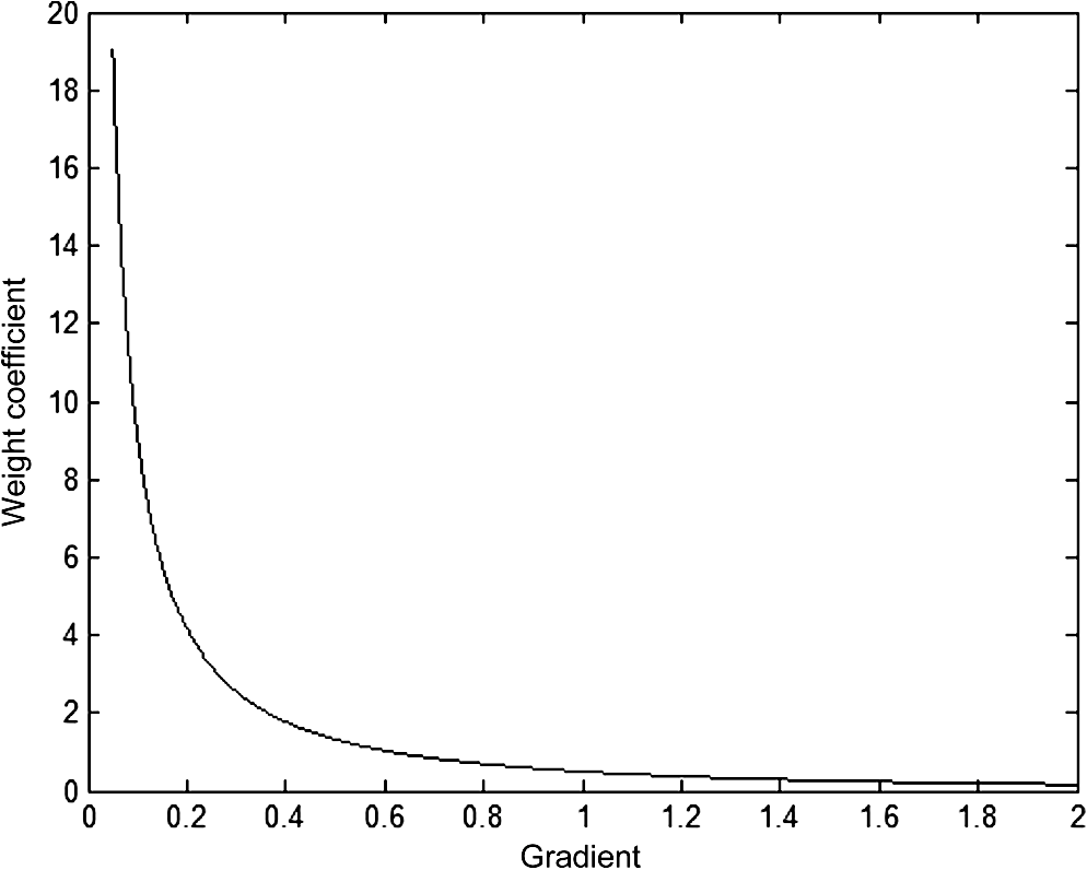
In the Mumford–Shah model,⁹ the $L_{2}$ -norm of the gradient is a smoothing function for segmentation. The diffusibility performances of this function along the tangent and normal directions are the same, i.e., $ρ_{T} = ρ_{N} = 1$ . The diffusion actions in the normal direction cross the edge; thus, this function cannot satisfy the second condition. To preserve the edge, Chan et al.¹⁸ proposed the total variation that the $L_{1}$ -norm of the gradient replaces the $L_{2}$ -norm. The performance along the normal direction is zero. It does not satisfy the first condition, which leads to a pseudoedge in the smoothing subregions.

Unfortunately, the above two conditions are incompatible. Compared with the piecewise smoothing functions of the Mumford–Shah model⁹ and total variation,¹⁸ we design an edge-preserving smoothing function for image segmentation.

Eq. (6)

f (| \nabla u |) = \ln (1 + | \nabla u |) .

The diffusibility performance in the tangent and normal directions are as follows:

Eq. (7)

ρ_{T} = \frac{1}{(1 + | \nabla u |) | \nabla u |}, ρ_{N} = - \frac{1}{{(1 + | \nabla u |)}^{2}} .

Inside the subregion where gradients are low,

\lim_{| \nabla u | \to 0} ρ_{T} = \infty

,

\lim_{| \nabla u | \to 0} ρ_{N} = - 1

; at the edge where gradients are strong,

\lim_{| \nabla u | \to \infty} ρ_{T} = \lim_{| \nabla u | \to \infty} ρ_{N} = 0

, and

\lim_{| \nabla u | \to \infty} \frac{ρ_{N}}{ρ_{T}} = - 1

(see Fig. 1). It is a compromise of two conditions on edge-preserving smoothing. This function preserves the edge and smooths the inhomogeneous subregion. Therefore, the edge-preserving smoothing model is given as

Eq. (8)

\inf_{u} {E^{(EP)} (u) = \frac{τ}{2} \int_{Ω} {(u - u_{0})}^{2} d x d y + \int_{Ω} \ln (1 + | \nabla u |) d x d y} .

Fig. 1

The diffusibility performance of this function. The solid and dash dot curve denote the diffusibility in the tangent and normal direction, respectively.

This problem allows for a unique solution characterized by the Euler–Lagrange equation:

Eq. (9)

τ (u - u_{0}) - div [\frac{\nabla u}{(1 + | \nabla u |) | \nabla u |}] = 0 .

To compute the smoothing component, we use a semi-implicit finite difference scheme. Let a set

Λ

is four neighbors region of the center pixel (

i, j

), and

p

is a member of set

Λ

, the approximation of Eq. (9) can be simply written as

Eq. (10)

u (i, j) = \frac{1}{τ + \sum_{p \in Λ} ω (p)} [τ u_{0} (i, j) + \sum_{p \in Λ} ω (p) u (p)],

where

τ

is the edge-preserving parameter, in other words, it is the weight coefficient of the center pixel. The

ω (p)

is the weight coefficient of the neighbor pixel

p

, the relationship between

ω (p)

and the gradient is shown in Fig. 2.

Eq. (11)

ω (p) = \frac{1}{[1 + | \nabla u (p) |] | \nabla u (p) |} .

Fig. 2

The weight coefficient of the neighbor pixel.

2.2.

Adaptive Edge-Preserving Smoothing

In traditional edge-preserving smoothing algorithms (i.e., TV¹⁸), the edge-preserving parameter $τ$ in Eq. (10) often is fixed by an artificial setting. If $τ ≫ ω (p)$ , then $u (i, j) \approx u_{0} (i, j)$ . The smoothing component contains the redundancy of inhomogeneous subregion, which causes the level set converge to local optima. If $τ ≫ ω (p)$ , the $u (i, j)$ approximates the weighted-mean of four neighborhood pixels. The edge of the smoothing component is blurred, the segmentation-curve is overconvergence. Above all, the fixed parameter cannot weigh up the edge-preserving and subregion smoothing according to local information of an image.

To solve the above problem, we analyze the two-clustering of the center pixel and four neighbors based on their possible spatial relationship.

• If four neighborhood pixels locate in the object region, the center pixel belongs to the object region according to the subregion connectivity.
• If the center pixel locates at the object boundaries, one of the following three cases applies:
- – One of the four neighbor pixels locates in background, others in an object region. There are $(\begin{matrix} 4 \\ 1 \end{matrix}) = 4$ kinds of situations.
- – Two of the four neighbor pixels locate in background and others in an object region, there are $(\begin{matrix} 4 \\ 2 \end{matrix}) = 6$ kinds of situations.
- – According to the continuity of the object contour, three or all of neighbor pixels cannot locate in the background.

The two-clustering of the center pixel and its four neighbors are shown in Fig. 3. Observed from Fig. 3, the edge-preserving parameter $τ$ is set as the medium of the weight coefficients of the center pixel and its four-neighbor:

Eq. (12)

τ = k \times medium {\frac{1}{[1 + | \nabla u_{0} (i, j) |] | \nabla u_{0} (i, j) |}, ω (p)} p \in Λ_{0},

where

k

is the constant, which normalizes parameter

τ

.

Fig. 3

The two-clustering of the center pixel and its four neighbors, the white and black circles denote object and background, respectively. (a) All pixels in the object region, (b) one of the four neighbor pixels locates in background and others in object region, and (c) two of the four neighbor pixels locate in background and others in object region.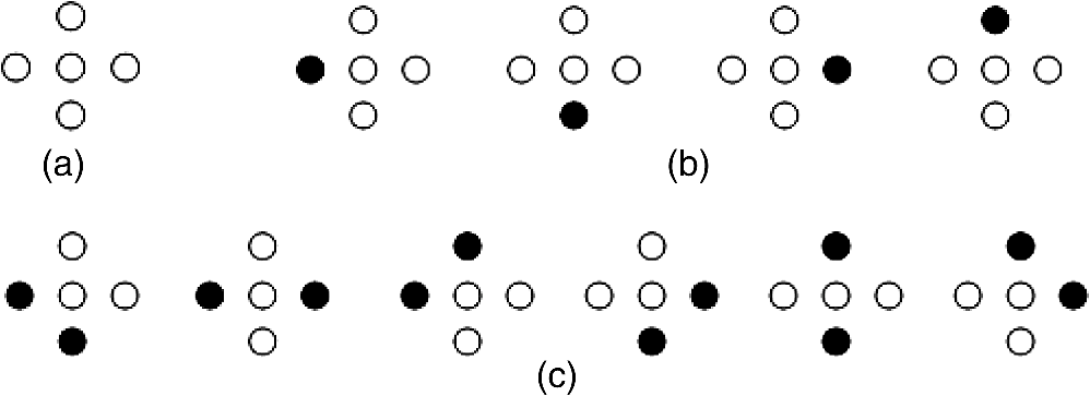

3. Segmentation Model

In terms of the analysis in Sec. 2, the segmentation model on the smoothing component is proposed as the following minimization problem:

Eq. (13)

\inf_{C} {E (u, C) = \int_{Ω} (u (x, y) - u_{0} {(x, y)}^{2} d x d y + \int_{Ω} \ln (1 + | \nabla u (x, y) |) d x d y + γ ‖ C ‖} .

During image segmentation, the curve may have a topological deformation (split or merge). To cope with this problem, active contours based on the level set are applied into image segmentation. The basic idea is to represent contours as the level set of an implicit function $φ (x, y)$ , i.e., $C = {(x, y) | φ (x, y) = 0}$ . The inside-region denotes ${(x, y) | φ (x, y) < 0}$ and outside-region is ${(x, y) | φ (x, y) > 0}$ . To simplify, both regions are approximated by the Heaviside function $H (φ)$ . The curve is represented as the Dirac measure $δ (φ)$ , which is the derivative of $H (φ)$ , where $H (φ)$ and $δ (φ)$ are defined as, respectively,

Eq. (14)

H (φ) = {\begin{cases} 1 & φ \geq 0 \\ 0 & φ < 0 \end{cases}, δ (φ) = \frac{d H (φ)}{d φ} .

However,

φ (x, y)

cannot satisfy the regularity condition

| \nabla φ | = 1

, the penalty term is introduced¹⁵

Eq. (15)

p (φ) = \frac{1}{2} \int_{Ω} {| \nabla φ - 1 |}^{2} d x d y .

Since the circumference and the area of the closed curve become smaller, the optimal segmentation curve is represented as

Eq. (16)

\inf_{φ} {ϵ (φ) = λ \int_{Ω} g δ (φ) | \nabla φ | d x d y + ν \int_{Ω} g H (- φ) d x d y + \frac{μ}{2} \int_{Ω} {| \nabla φ - 1 |}^{2} d x d y},

where

λ

and

ν

are the weight of the circumference and area of curve, respectively, and

g

is the edge indicator function of the smoothing component

Eq. (17)

g = {(1 + | \nabla u |)}^{- 1} .

If the level set curve locates in where the gradients are low, the edge indicator function is almost the maximum of the entire image. Otherwise, the edge indicator function is the minimum, and the level set curve convergence to the boundary.

Consequently, we incorporate the edge-preserving smoothing model into the above segmentation model, and construct the energy function of the edge-preserving smoothing segmentation model.

Eq. (18)

\inf_{φ} {E (u, φ) = \int_{Ω} {[u (x, y) - u^{0} (x, y)]}^{2} d x d y + \frac{τ}{2} \int_{Ω} \ln [1 + | \nabla u (x, y) |] d x d y + λ \int_{Ω} g δ (φ) | \nabla φ | d x d y + ν \int_{Ω} g H (- φ) d x d y + \frac{μ}{2} \int_{Ω} {| \nabla φ - 1 |}^{2} d x d y} .

To minimize the function

E (u, φ)

, we denote the Gateaux derivative¹⁹ of the function

E (φ, u)

as

\partial E (φ, u) / \partial φ

. By calculating variations, the Gateaux derivative of the function

E (φ, u)

in Eq. (18) can be written as

Eq. (19)

\frac{\partial E (u, φ)}{\partial φ} = - μ [Δ φ - div (\frac{\nabla φ}{| \nabla φ |})] - λ δ (φ) div (g \frac{\nabla φ}{| \nabla φ |}) - ν g δ (φ),

where

Δ

is the Laplacican operator. Therefore,

φ

satisfies the Euler–Lagrange equation. By introducing an artificial temporal variable

t

, we use the steepest descent process to get minimization of the function

E (u, φ)

, whose gradient flow is

Eq. (20)

\frac{\partial φ}{\partial t} = μ [Δ φ - div (\frac{\nabla φ}{| \nabla φ |})] + λ δ (φ) div (g \frac{\nabla φ}{| \nabla φ |}) + ν g δ (φ) .

4. Implementation

In Eq. (20), the Dirac measure $δ (φ)$ is noncontinuous. When calculating the level set, take continuous $δ_{a} (φ)$ ( $a = 1.5$ ) instead of $δ (φ)$

Eq. (21)

δ_{a} (φ) = {\begin{cases} 0 & | φ | > a \\ \frac{1}{2 a} [1 + \cos (\frac{π φ}{a})] & | φ | \leq a \end{cases} .

In this paper, the $\partial φ / \partial t$ is approximated by the forward difference, and the $\nabla φ$ is approximated by the central difference. The approximation of Eq. (20) for the smoothing component $u^{m}$ can be simply written as

Eq. (22)

\frac{φ_{i, j}^{k + 1} - φ_{i, j}^{k}}{Δ t} = μ [Δ (φ_{i, j}^{k}) - div (\frac{\nabla φ_{i, j}^{k}}{| \nabla φ_{i, j}^{k} |})] + λ δ_{a} (φ_{i, j}^{k}) div (g_{i, j}^{m} \frac{\nabla φ_{i, j}^{k}}{| \nabla φ_{i, j}^{k} |}) + ν g_{i, j}^{m} δ_{a} (φ_{i, j}^{k}),

where,

Δ t

is the time step, and

g_{i, j}^{m}

is edge indicator function of the smoothing component

u^{m}

.

u^{m}

is calculated by the fixed-point iteration algorithm

Eq. (23)

u_{i, j}^{m} = \frac{1}{τ^{m} + \sum_{p \in Λ_{0}} ω^{m} (p)} [\sum_{p \in Λ_{0}} ω^{m} (p) u^{m - 1} (p) + τ^{m} u_{0} (i, j)] .

For Eq. (23), the smoothing component converges to the mean of the initial image without constraint conditions, which leads to the difference between the features of the object and the surrounding region not being significant. To avoid this phenomenon, we present the confidence level of segmented subregions on two adjacent iterations of the smoothing component, which is defined as following:

Eq. (24)

P r = \frac{card (A^{m} \cap A^{m - 1})}{\max [card (A^{m}), card (A^{m - 1})]} .

Here the set

A^{m}

and

A^{m - 1}

represent the segmented subregions

[(x, y) | φ (x, y) \leq 0]

for the smoothing component

u^{m}

and

u^{m - 1}

, respectively. When the confidence level satisfies the following condition, the smooth is terminated:

Eq. (25)

P r \geq T,

where

T

is the threshold of the regional confidence level.

The steps of image segmentation (output)

{Initial: $k, λ, μ, ν, Δ t, T, φ^{0} (x, y)$ and $u^{0} = u_{0}$ }

N is the iterative number of image smoothing

Begin

N:= 0;

Repeat

Computing the weight coefficient $ω (p)$ of smoothing component $u^{N}$ uses:

Eq. (26)

ω^{N} (p) = \frac{1}{(1 + | \nabla u^{N - 1} (p) |) | \nabla u^{N - 1} (p) |} .

Computing the edge-preserving parameter $τ$ :

Eq. (27)

τ^{N} = k \times medium {\frac{1}{(1 + | \nabla u_{0} (i, j) |) | \nabla u_{0} (i, j) |}, ω^{N} (p)} p \in Λ_{0} .

Computing the smoothing component $u^{N}$ uses:

Eq. (28)

u_{i, j}^{N} = \frac{1}{τ^{N} + \sum_{p \in Λ_{0}} ω^{N} (p)} [\sum_{p \in Λ_{0}} ω^{N} (p) u^{N - 1} (p) + τ^{N} u_{0} (i, j)] .

Computing the edge indicator function of the smoothing component $u^{N}$ uses:

Eq. (29)

g (u^{N}) = \frac{1}{1 + | \nabla u^{N} |} .

Segmentation of the smoothing component $u^{N}$ uses: Eq. (22)

Until

The convergence condition: Eq. (25)

Output: the result of segmentation.

End

5. Experimental Results

5.1.

Implementation Details

The experiments are conducted using VC 6.0 on a PC with Intel-Core i5 CPU @ 3.40 GHz and 4 GB of RAM without any particular code optimization. During the implementation of the proposed model, we used the parameters $λ = 5.0$ , $μ = 0.04$ , $ν = 3.0$ and time step $Δ t = 5.0$ for all experiments. Here, we propose the following functions as the initial function $φ^{0} (x, y)$ . Let $\partial Ω_{0}$ be all the points on the boundaries of $Ω_{0}$ which is a subset in the image domain $Ω$ . Then, the initial function $φ^{0} (x, y)$ is defined as

Eq. (30)

φ^{0} (x, y) = {\begin{cases} - ξ & (x, y) \in Ω_{0} - \partial Ω_{0} \\ 0 & (x, y) \in \partial Ω_{0} \\ ξ & (x, y) \in Ω - Ω_{0} \end{cases},

where

ξ

is a constant. We suggest to choose

ξ

larger than

2 a

, where

a

is the width in the definition of the regularized Dirac function

δ_{a} (φ)

in Eq. (21).

In this paper, we use three universally agreed on, standard, and easy-to-understand measures for evaluating a segmentation model, those are precision, recall, and F-measure. The first two evaluation metrics are based on the overlapping area between ground truth and segmentation regions. Usually, neither precision nor recall can comprehensively evaluate the quality of segmentation. So the F-measure is proposed as a harmonic mean of them. For a segmentation object region, we can convert it to a binary mask $M$ and compute precision and recall by comparing $M$ with ground-truth $G$

Eq. (31)

precision = \frac{| M \cap G |}{| M |}, recall = \frac{| M \cap G |}{| G |}, F - measure = \frac{2 \times precision \times recall}{precision + recall} .

5.2.

Discussion

The image is smoothed using the edge-preserving smoothing model in the proposed model, so the segmentation performance depends on the parameter $k$ in Eq. (12). To analyze the relationship between $k$ and the scores of image segmentation (precision, recall, and F-measure), a $480 \times 320$ -pixel image with grass and sand in the Berkeley segmentation database is smoothed with different parameter $k$ , and the results of segmentation are shown in Fig. 4. The initial curve and ground truth are represented as a red rectangle and yellow curve, respectively, in the top left-hand corner subimage of Fig. 4.

Fig. 4

The results of segmentation, edge indicator functions, and smoothing components with different parameter $k$ . (a) The flowerbed, (b) the edge indicator function, and (c) the cartoon component. Row 1: original images and initial curves, rows 2 to 5: the results of segmentation, edge indicator function, and smoothing component using 0.005, 0.05, 0.2, 0.25, and 0.5, respectively.

As illustrated in the second row, the subregion pixels close to constant and the edge are blurred by this smoothing algorithm with $k = 0.005$ . The blurred edge leads to the over-convergence of the level set, which results in parts of the object region pixels being mistaken as the background. Thus, the recall is low at 0.862. The precision and the F-measure are 0.995 and 0.915, respectively.

As illustrated in the last row, when $k = 0.5$ , the smoothing component contains remnants of an inhomogeneous subregion, which leads to the level set convergence at the local optimum. The precision is low, and the F-measure is 0.848.

Figure 5 shows CPU times and scores of the segmentation on Fig. 4 using this model with different parameters $k$ . While $k$ is smaller, the precision, recall, and F-measure of the segmentation are lower and the CPU time is shorter.

Fig. 5

The CPU time (in seconds) and score of segmentation in Fig. 4. (a) The CPU time of the segmentation using the different parameter $k$ . (b) The red, green, and blue curves show the F-measure, precision, and recall of the segmentation the different parameter using the different parameter $k$ , respectively.

If $k$ is large, the remnants inhomogeneous subregion leads to the level set’s fast convergence at the local optimum. When $k \in [0.05, 0.18]$ , this model preserves the edge and smooths the inhomogeneous subregion. The maximum difference of the F-measure is 0.005, e.g., the F-measures of the segmentation with $k = 0.05$ and 0.18 are 0.98 and 0.975, respectively.

In this model, the smooth components converge to the mean of the image without constrained conditions, which leads to the difference between the feature of the object and that of the surrounding region not being significant. To avoid this, we use the threshold of segmented subregions confidence level. To validate how the threshold affects the segmentation performance, a $480 \times 320$ -pixel potted-tree image of the Berkeley segmentation database, in which some subregions are inhomogeneous (crown of the tree), is segmented with different thresholds.

The segmentation results are shown in Fig. 6. The initial curve and the ground truth, represented as a red rectangle and blue curve, respectively, are shown in Fig. 6(a). The smoothing component retains an inhomogeneous subregion by this smoothing algorithm using the threshold $T = 0.95$ , which leads to parts of background region pixels being mistaken as the object [shown in Fig. 6(b)]. The precision of segmentation is 0.937, and the F-Measure is 0.959. When $T = 0.99$ , the weak edge is smoothed [see the inside circle in Fig. 6(f)] and the computation time is longer. The F-measure, recall, and precision are 0.978, 0.961, and 0.997. The CPU time and score of segmentation using this model with the different threshold are shown in Fig. 7. As shown in Fig. 7, when the threshold increases, the computation time using this model is longer. If the threshold closes to one, the F-measures of segmentation descend.

Fig. 6

The results of segmentation with different thresholds. (a) Initial curve and the ground truth and (b)–(f) the results of segmentation using different thresholds 0.95, 0.96, 0.97, 0.98, and 0.99, respectively.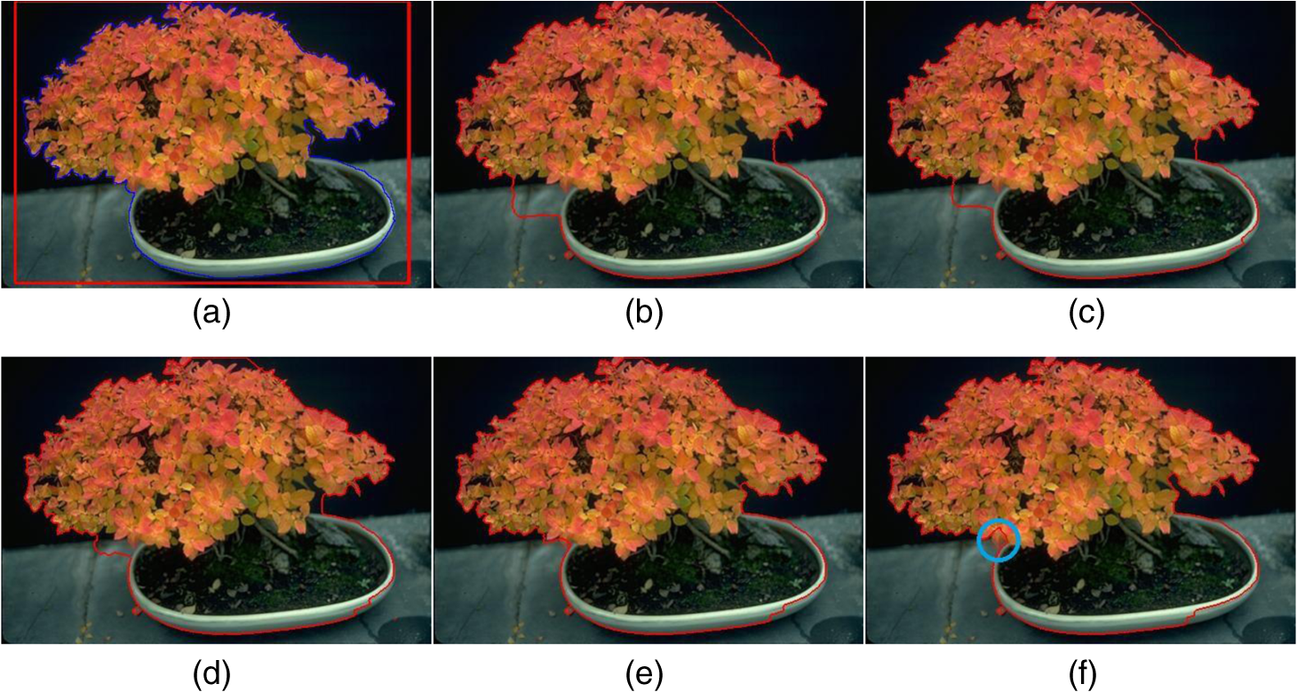

Fig. 7

The CPU time and score of segmentation in Fig. 6. (a) The CPU time of the segmentation using the different threshold $T$ . (b) The red, green, and blue curves show the F-measure, precision, and recall of segmentation with the different threshold $T$ , respectively.

The parameter $k$ is the constant that normalizes parameter $τ$ and parameter $T$ is the threshold of the regional confidence level. In order to preserve the edge and smooth the inhomogeneous subregion, we suggest to choose $k = 0.05$ and $T = 0.98$ .

5.3.

Segmentation Algorithm Comparisons

To test segmentation performance using the proposed method on real images with slightly inhomogeneous subregions, the experiments are carried on to compare with the Li’s model,¹⁵ TB model,²⁰ and the CV model.⁸ The choice of these algorithms is motivated by the following reasons: these four algorithms all employ the level set. Li’s model and TB model exploited the edge feature; the image is preprocessed by the Gaussian filter and the classical TV, respectively. In the TB model, the TV smoothing and the smoothing-component segmentation are individual steps. The number of iterations was not taken into consideration. The CV model uses the regional characteristics of the subregion to represent the object as the mean of the subregion. The different sizes of images are segmented, which are from the International web and the Berkeley segmentation database. The partial results are shown is shown in Fig. 8. The effects of the four algorithms on the homogeneous image are almost similar, such as Fig. 8(a). For the image with weak edges [i.e., Fig. 8(b)], the results of segmentation using the proposed method and TB model are better than those of the other two models. Segmentation performance using the CV model is poor for inhomogeneous subregions, e.g., Fig. 8(c), and the F-measure is 0.812. This is the reason that the intensity mean of a subregion indicates the region.

Fig. 8

Comparison of the proposed method with Li’s model¹³ and the TB model,²⁰ and the CV model⁸ on real images. (a) The lotus, (b) the eagles, and (b) the butterfly. Row 1: original images and initial curves, row 2: segmentation results of the CV, row 3: the segmentation results of Li’s model, row 4: segmentation results of the TB model, row 5: the segmentation results of the proposed model, and row 6: the ground truth.

However, the effect of the proposed method for images with a seriously inhomogeneous region, such as the images in Fig. 9, is better than that of the other three models.

Fig. 9

Comparison of the proposed method with Li’s models¹³ and the CV model⁸ on real images with serious in-homogeneity. (a) The blossom, (b) the viburnum, and (c) the cycas. Row 1: original images and initial curves, row 2: segmentation results of the CV model, row 3: the segmentation results of Li’s model, row 4: segmentation results of the TB model, row 5: the segmentation results of the proposed model, and row 6: the ground truth.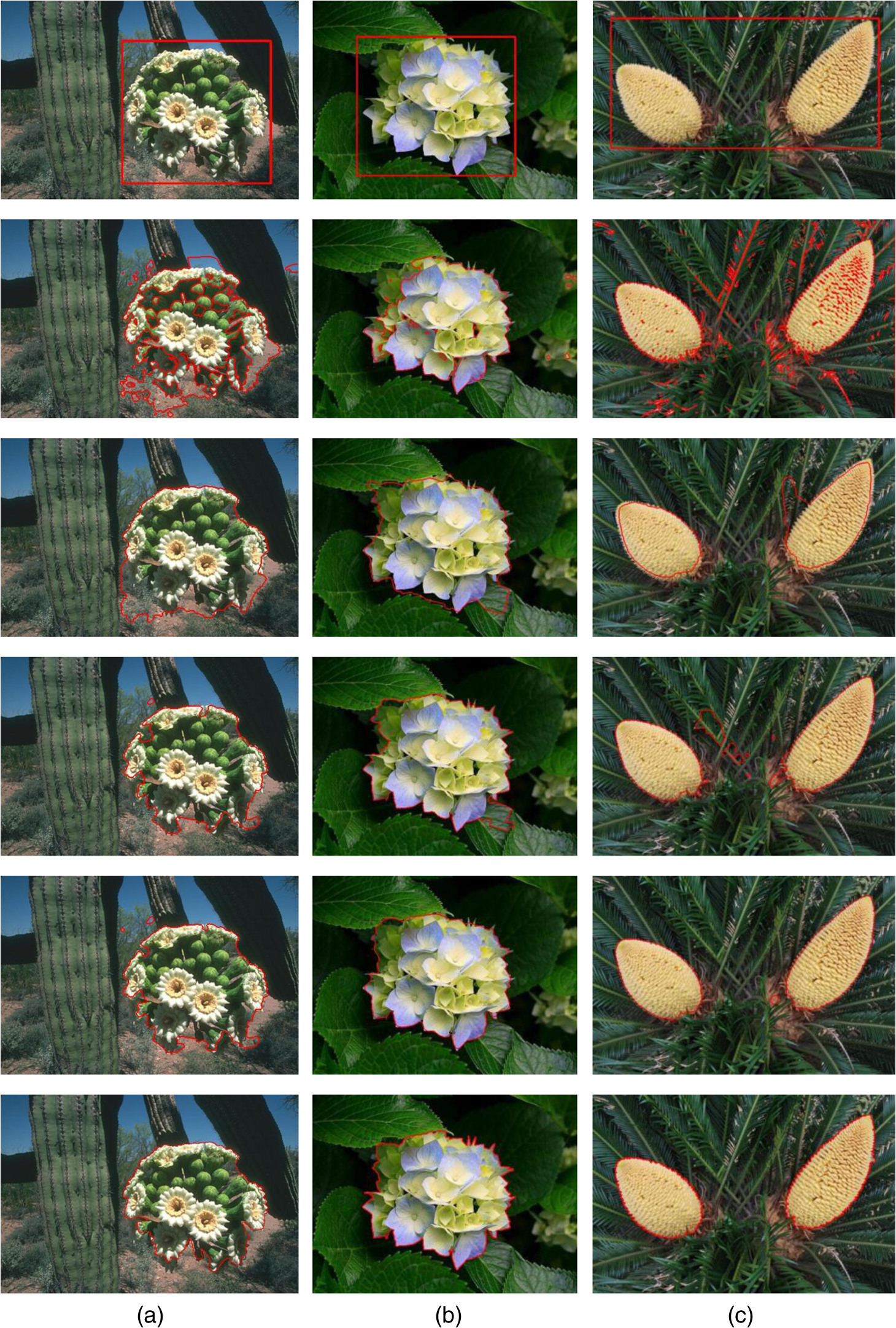

The objector region is divided into many subregions using the CV model,⁸ which is that the object region contains many subregions with different intensities. The Li’s model¹³ avoids oversegmentation, but the segmentation curve is far away from the true boundaries where gradients are low. The positional accuracy using the TB model²⁰ is higher than that of Li’s model, there is oversegmentation, as shown in Fig. 9(c). The segmentation curve using the proposed method cannot locate at the object boundaries with weak edges [i.e., Fig. 9(a)]. For the images in Figs. 8 and 9, the CPU time and scores of segmentation are given in Table 1.

Table 1

The comparison of CPU time and scores of segmentation in Figs. 8 and 9.

Method	Image and its size
	Fig. 8(a)	Fig. 8(b)	Fig. 8(c)	Fig. 9(a)	Fig. 9(b)	Fig. 9(c)
	320×240	480×320	580×385	480×320	512×384	600×392
Proposed method
Precision	0.995	0.996	0.999	0.932	0.989	0.994
Recall	0.943	0.863	0.967	0.948	0.965	0.950
F-measure	0.969	0.925	0.983	0.940	0.977	0.972
CPU time (s)	6.006	8.985	9.672	11.66	22.17	39.34
Li’s model
Precision	0.985	0.981	0.986	0.813	0.914	0.928
Recall	0.953	0.866	0.989	0.967	0.960	0.857
F-measure	0.968	0.920	0.988	0.883	0.937	0.891
CPU time (s)	3.666	9.579	8.892	8.277	9.406	28.97
TB model
Precision	0.988	0.996	0.998	0.936	0.949	0.921
Recall	0.947	0.862	0.968	0.929	0.957	0.952
F-measure	0.967	0.924	0.983	0.932	0.953	0.936
CPU time (s)	4.509	8.799	9.454	9.771	11.62	25.45
CV model
Precision	0.999	0.891	0.999	0.756	0.995	0.889
Recall	0.946	0.932	0.684	0.696	0.828	0.922
F-measure	0.972	0.911	0.812	0.724	0.904	0.905
CPU time (s)	3.182	6.365	9.313	3.559	9.016	17.55

Compared to the effect of Li’s model, the TB model and the CV model on real images with inhomogeneous subregions and weak edges, the effect of the proposed method is better. Nevertheless, the computation time using the proposed method is costly, which is the reason that this method uses iteration smoothing to deal with the inhomogeneous subregion. However, Li’s model uses the Gaussian smoothing only one time, and the CV model does not smooth the image. For images of the same size, the iterative number mainly depends on the region’s inhomogeneous degree, such as for images in Figs. 8(b) and 9(a), the CPU time using the proposed method is 8.985 and 11.66 s, respectively.

To test the proposed method’s robustness against noise, segmented experiments on a $320 \times 240$ degraded image with additive white noise are conducted and compared with Li’s model,¹⁵ the TB model,²⁰ and the CV model.⁸ Partial results are shown in Fig. 10. With the PSNR decreasing, the isotropic diffusion in Li’s model blurs the object contour, and the fixed variance of Gauss kernel function cannot remove all kinds of noise. The level set curve could not locate accurately. The subregions in the object are separated using the CV model. Furthermore, the results of segmentation become terrible with lower PSNR. Compared to the ground truth, the positional accuracy of the segmentation curve using the proposed method is higher than that of the TB model. The edge-preserving parameter preserves edges and smooths subregions, according to local information. The scores of different models with different PSNR are shown in Table 2.

Fig. 10

Comparison of the proposed method with Li’s models¹³ and the CV model⁸ on real images with noise. (a) The original image, (b) noisy image with PSNR=23.4, and (c) noisy image with PSNR=18.8. Row 1: noisy images and initial curves, row 2: segmentation results of the CV model, row 3: the segmentation results of Li’s model, row 4: segmentation results of the TB model, row 5: the segmentation results of the proposed model, and row 6: the ground truth.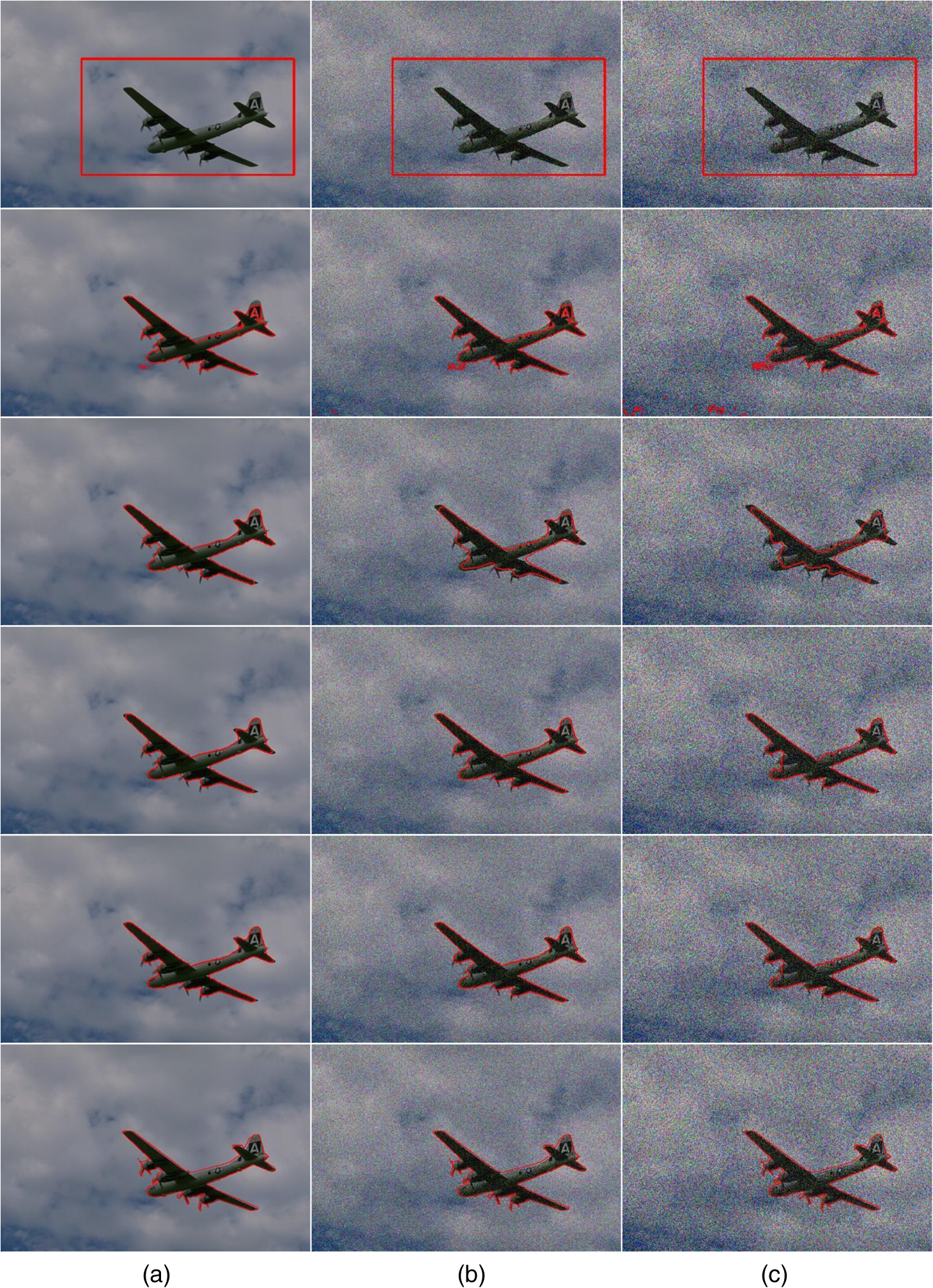

Table 2

The scores of different algorithms on noisy images (where Pre, Rec, and F-M denote precision, recall, and F-measure, respectively).

PSNR (dB)	Model
	Proposed method			Li model			TB model			CV model
	Pre	Rec	F-M	Pre	Rec	F-M	Pre	Rec	F-M	Pre	Rec	F-M
29.9	0.992	0.838	0.909	0.915	0.717	0.804	0.989	0.827	0.901	0.976	0.785	0.870
23.4	0.992	0.838	0.909	0.901	0.719	0.799	0.988	0.812	0.891	0.967	0.785	0.866
22.3	0.989	0.831	0.903	0.891	0.722	0.797	0.987	0.828	0.901	0.965	0.786	0.866
21.7	0.988	0.817	0.894	0.868	0.722	0.788	0.979	0.821	0.893	0.945	0.790	0.860
20.1	0.981	0.826	0.897	0.857	0.726	0.786	0.974	0.812	0.886	0.926	0.792	0.853
19.5	0.986	0.826	0.899	0.847	0.725	0.781	0.971	0.817	0.887	0.905	0.791	0.844
18.8	0.981	0.819	0.893	0.837	0.731	0.78	0.963	0.831	0.892	0.874	0.791	0.830
17.6	0.973	0.839	0.901	0.781	0.732	0.756	0.955	0.835	0.891	0.855	0.793	0.823
16.7	0.951	0.818	0.879	0.759	0.731	0.745	0.915	0.824	0.867	0.814	0.793	0.803
15.4	0.942	0.817	0.875	0.637	0.729	0.679	0.855	0.817	0.836	0.792	0.794	0.793
14.8	0.911	0.831	0.869	0.518	0.732	0.607	0.801	0.786	0.793	0.733	0.796	0.763
12.9	0.904	0.833	0.867	0.445	0.735	0.554	0.716	0.791	0.752	0.686	0.801	0.739
Original image	0.992	0.838	0.909	0.915	0.717	0.804	0.989	0.827	0.901	0.976	0.785	0.870
Mean	0.968	0.829	0.892	0.782	0.726	0.745	0.929	0.818	0.868	0.878	0.791	0.829
Variance	0.031	0.009	0.015	0.155	0.006	0.081	0.086	0.015	0.047	0.097	0.005	0.043

From Table 2, with decreasing image quality, the precise and the F-measure of these four segmentation models reduce. The variance of F-measure using the proposed method, Li’s model,¹⁵ the TB model,²⁰ and the CV model⁸ are 0.015, 0.081, 0.047, and 0.043, respectively. The variance of F-measure using the proposed method is smaller than those of other three models. The mean of the F-measure using the proposed method, Li’s model, the TB model, and the CV model are 0.892, 0.745, 0.878, and 0.829, respectively. The mean of F-measure using the proposed method is higher than those of other three models. It shows that our proposed method is insensitive to noise. Although the proposed method is insensitive to noise, the computer time is longer than that of other three models. The CPU time comparison of segmentation on an image with noise is shown in Table 3.

Table 3

The comparison of CPU time (in seconds) with noisy images.

PSNR (dB)	29.9	23.4	22.3	21.7	20.1	19.5	18.8	17.6	16.7	15.4	14.8	12.9	Original image
Proposed model	9.55	10.7	11.3	13.3	14.5	14.9	17.4	17.7	17.9	18.2	19.5	20.9	9.34
TB model	8.54	9.8	10.3	10.4	10.9	10.9	11.2	12.6	13.1	13.9	15.3	16.2	8.11
Li’s model	4.23	4.67	4.78	5.16	5.89	6.79	7.45	7.98	8.39	9.43	9.96	10.67	4.12
CV model	3.48	3.61	4.07	4.49	5.32	6.21	6.53	7.23	7.41	7.89	8.13	8.98	3.31

To test robustness against salt-and-pepper noise of the proposed method, segmented experiments on a $500 \times 375$ degraded image are conducted and compared with Li’s model,¹⁵ the TB model,²⁰ and the CV model.⁸ Partial results are shown in Fig. 11. The linear smoothing (Gauss smoothing) cannot effectively remove salt-and-pepper noise, so Li’s segmentation curve could not converge with the object contour, and the F-Measure is 0.849. The CV model could converge with the object contour, but oversegmentation exists, the F-measure is 0.909, and the recall is 0.853; nonlinear smoothing (TV or median filter) can effectively remove the salt-and-pepper noise, the precisions of the proposed model and the TB model are 0.994 and 0.986, respectively. In the TB model, the TV smoothing and the smoothing-component segmentation are individual steps. It could not adaptively adjust the relationship between the number of smoothing iteration and region-confidence level. The F-measure of the proposed method is 0.98, and 0.021 higher than that of TB model.

Fig. 11

Comparison of the proposed method with Li’s models¹³ and the CV model⁸ on real images with salt-and-pepper noise. (a) Initial curves, (b) the ground truth, (c) the proposed model, (d) the segmentation results of the CV model, (e) the segmentation results of the Li’s model, and (f) segmentation results of the TB model.

6. Concluding Remarks

To improve segmentation performance of the active contour model on real images, we propose an image segmentation model based on edge-preserving smoothing. Compared to Li’s model, the CV model, and TB model on real images, the experimental results have shown that this method is insensitive to noise and can deal with inhomogeneous subregions. However, the proposed edge-preserving smoothing just retains the edge information, but could not sharpen weak edges. Thus, the proposed method cannot precisely locate the object contour formed by a weak edge. Furthermore, the computational cost is high. In the future, we plan to design an efficient model to sharpen the weaken edge.

Acknowledgments

This work was supported by the Sichuan Province Natural Science Foundation of China (Grant No. 2013SZ0157). The author Kun He and the author Dan Wang give the improved algorithm and the structure of the article. The algorithm implementation and the article writing are collaborative efforts. Partial experimental results in the article are given by Xiuqing Zheng.

References

1.

Y. K. Sen et al., “Image segmentation methods for intracranial aneurysm haemodynamic research,” J. Biomech., 47 (5), 1014 –1019 (2014). http://dx.doi.org/10.1016/j.jbiomech.2013.12.035 JBMCB5 0021-9290 Google Scholar

2.

R. C. Zhao and Y. D. Ma, “A novel region segmentation algorithm with neural network for segmented image coding,” Acta Electron. Sin., 42 (7), 1277 –1283 (2014). http://dx.doi.org/10.3969/j.issn.0372-2112.2014.07.006 TTHPAG 0372-2112 Google Scholar

3.

M. Caon et al., “Computer-assisted segmentation of CT images by statistical region merging for the production of voxel models of anatomy for CT dosimetry,” Australas. Phys. Eng. Sci. Med., 37 (2), 393 –403 (2014). http://dx.doi.org/10.1007/s13246-014-0273-x Google Scholar

4.

X. Yang et al., “Improving level set method for fast auroral oval segmentation,” IEEE Trans. Image Process., 23 (7), 2854 –2865 (2014). http://dx.doi.org/10.1109/TIP.2014.2321506 IIPRE4 1057-7149 Google Scholar

5.

J. B. Shen, Y. F. Du and X. L. Li, “Interactive segmentation using constrained Laplacian optimization,” IEEE Trans. Circuits Syst. Video Technol., 24 (7), 1086 –1099 (2014). http://dx.doi.org/10.1109/TCSVT.2014.2302545 ITCTEM 1051-8215 Google Scholar

6.

M. W. Khan, “A survey: image segmentation techniques,” Int. J. Future Comput. Commun., 3 (2), 89 –93 (2014). http://dx.doi.org/10.7763/IJFCC.2014.V3.274 Google Scholar

7.

L. Wang et al., “Joint segmentation and recognition of categorized objects from noisy web image collection,” IEEE Trans. Image Process., 23 (9), 4070 –4086 (2014). http://dx.doi.org/10.1109/TIP.2014.2339196 IIPRE4 1057-7149 Google Scholar

8.

T. F. Chan and L. Vese, “Active contours without edges,” IEEE Trans. Image Process., 10 (2), 266 –277 (2001). http://dx.doi.org/10.1109/83.902291 IIPRE4 1057-7149 Google Scholar

9.

D. Mumford and J. Shah, “Optimal approximations of piecewise smooth functions and associated variational problems,” Commun. Pure Appl. Math., 42 (5), 577 –685 (1989). http://dx.doi.org/10.1002/(ISSN)1097-0312 CPMAMV 0010-3640 Google Scholar

10.

A. Tsai et al., “Curve evolution implementation of the mumford-shah functional for image segmentation, denoising, interpolation, and magnification,” IEEE Trans. Image Process., 10 (8), 1169 –1186 (2001). http://dx.doi.org/10.1109/83.935033 Google Scholar

11.

C. Li et al., “Implicit active contours driven by local binary fitting energy,” in Proc. IEEE Conf. on Computer Vision and Pattern recognition, 1 –7 (2007). http://dx.doi.org/10.1109/CVPR.2007.383014 Google Scholar

12.

Y. Peng et al., “Active contours driven by normalized local image fitting energy,” J. Syst. Eng. Electron., 25 (2), 307 –313 (2014). http://dx.doi.org/10.1109/JSEE.2014.00035 Google Scholar

13.

H. Y. Jiang and R. J. Feng, “Image segmentation method research based on improved variational level set and region growth,” Acta Electron. Sin., 40 (8), 1659 –1664 (2012). http://dx.doi.org/10.3969/j.issn.0372-2112.2012.08.026 TTHPAG 0372-2112 Google Scholar

14.

D. Kong and G. Wang, “Region-similarity based active contour model for SAR image segmentation,” J. Comput.-Aided Des. Comput. Graphics, 22 (9), 1554 –1560 (2010). Google Scholar

15.

C. Li et al., “Level set evolution without re-initialization: a new variational formulation,” in the Proc. of the 2005 IEEE Computer Society Conf. on Computer Vision and Pattern Recognition, 430 –436 (2005). http://dx.doi.org/10.1109/CVPR.2005.213 Google Scholar

16.

Q. Wen et al., “Decomposition and active contour method for medical noise image segmentation,” J. Comput.-Aided Des. Comput. Graphics, 23 (11), 1882 –1889 (2011). Google Scholar

17.

S. Y. Yeo et al., “Segmentation of biomedical images using active contour model with robust image feature and shape prior,” Int. J. Numer. Methods Biomed. Eng., 30 (2), 232 –248 (2014). http://dx.doi.org/10.1002/cnm.2600 Google Scholar

18.

T. F. Chan, S. Osher and J. H. Shen, “The digital TV filter and nonlinear denoising,” IEEE Trans. Image Process., 10 (2), 231 –241 (2001). http://dx.doi.org/10.1109/83.902288 IIPRE4 1057-7149 Google Scholar

19.

L. Evans, Partial Differential Equations, American Mathematical Society, Providence (1998). Google Scholar

20.

K. He, X. Q. Zheng and Y. L. Zhang, “Image segmentation on texture blurring,” J. Sichuan Univ., 47 (4), 111 –117 (2015). http://dx.doi.org/10.15961/j.jsuese.2015.04.016 Google Scholar

Biography

Kun He received his PhD in electrical and computer engineering from Sichuan University in 2006. Since 2006, he has been working as a professor research fellow in the School of Computer Science, Sichuan University. His research interests include pattern recognition, computer vision, and image processing.

Dan Wang received the bachelor's degree in software engineering from Sichuan University in 2014. She is currently a graduate student of the software engineer, the Key National Defense Laboratory of Visual Synthesis Graphic and Image, Sichuan University. Her major work was pattern recognition, image processing, and medical image analysis.

Xiuqing Zheng received her PhD in computer science and technology, Sichuan University. Currently, she served as the associate dean of Applied Technology College in Sichuan Normal University. Her research interests include intelligent information processing and image processing. She has undertaken and presided over many scientific and technological projects.

CC BY: © The Authors. Published by SPIE under a Creative Commons Attribution 4.0 Unported License. Distribution or reproduction of this work in whole or in part requires full attribution of the original publication, including its DOI.

Citation Download Citation

Kun He, Dan Wang, and Xiuqing Zheng "Image segmentation on adaptive edge-preserving smoothing," Journal of Electronic Imaging 25(5), 053022 (4 October 2016). https://doi.org/10.1117/1.JEI.25.5.053022

Published: 4 October 2016

Access the abstract

JOURNAL ARTICLE
14 PAGES

DOWNLOAD PAPER SAVE TO MY LIBRARY

GET CITATION

CITATIONS

Cited by 4 scholarly publications.

Explore citations on Lens.org

KEYWORDS

Image segmentation

Lithium

Image processing algorithms and systems

Performance modeling

Statistical modeling

Diffusion

Gaussian filters

1.

Introduction

2.

Proposed Edge-Preserving Model

Eq. (1)

Eq. (2)

Eq. (3)

2.1.

Edge-Preserving Smoothing

Eq. (4)

Eq. (5)

Eq. (6)

Eq. (7)

Eq. (8)

Fig. 1

Eq. (9)

Eq. (10)

Eq. (11)

Fig. 2

2.2.

Adaptive Edge-Preserving Smoothing

Eq. (12)

Fig. 3

3.

Segmentation Model

Eq. (13)

Eq. (14)

Eq. (15)

Eq. (16)

Eq. (17)

Eq. (18)

Eq. (19)

Eq. (20)

4.

Implementation

Eq. (21)

Eq. (22)

Eq. (23)

Eq. (24)

Eq. (25)

Eq. (26)

Eq. (27)

Eq. (28)

Eq. (29)

5.

Experimental Results

5.1.

Implementation Details

Eq. (30)

Eq. (31)

5.2.

Discussion

Fig. 4

Fig. 5

Fig. 6

Fig. 7

5.3.

Segmentation Algorithm Comparisons

Fig. 8

Fig. 9

Table 1

Fig. 10

Table 2

Table 3

Fig. 11

6.

Concluding Remarks

Acknowledgments

References

Biography

Show All Keywords

Keywords/Phrases

Search In:

Publication Years