Automatic age and gender classification using supervised appearance model

Ali Maina Bukar; Hassan Ugail; David Connah

doi:10.1117/1.JEI.25.6.061605

1 August 2016 Automatic age and gender classification using supervised appearance model

Ali Maina Bukar, Hassan Ugail, David Connah

Author Affiliations +

Journal of Electronic Imaging, Vol. 25, Issue 6, 061605 (August 2016). https://doi.org/10.1117/1.JEI.25.6.061605

Abstract

Age and gender classification are two important problems that recently gained popularity in the research community, due to their wide range of applications. Research has shown that both age and gender information are encoded in the face shape and texture, hence the active appearance model (AAM), a statistical model that captures shape and texture variations, has been one of the most widely used feature extraction techniques for the aforementioned problems. However, AAM suffers from some drawbacks, especially when used for classification. This is primarily because principal component analysis (PCA), which is at the core of the model, works in an unsupervised manner, i.e., PCA dimensionality reduction does not take into account how the predictor variables relate to the response (class labels). Rather, it explores only the underlying structure of the predictor variables, thus, it is no surprise if PCA discards valuable parts of the data that represent discriminatory features. Toward this end, we propose a supervised appearance model (sAM) that improves on AAM by replacing PCA with partial least-squares regression. This feature extraction technique is then used for the problems of age and gender classification. Our experiments show that sAM has better predictive power than the conventional AAM.

1. Introduction

The human face conveys much information, which people have a remarkable ability to extract, identify, and interpret. Age and gender are known to influence the structure and appearance of the face, and human observers can reliably infer both. Recently, there has been an increase in the development of automatic facial analysis techniques with a view for developing machine-based systems that mimic these abilities of the human visual system. Both being demographic attributes of the human face, they play important roles in real-life applications that include biometrics, demographic studies, targeted advertisements, human–computer interaction systems, and access control. With much progress in automatic face detection and recognition, much research is now focused on automatic demographic identification.

Interestingly, research has shown that age estimation and classification are affected by gender differences¹ as well as actual age.² Indeed, both facial age and gender classifications have been studied together as related problems.³^–⁵ Similarly, the two problems have been tackled simultaneously in other fields such as automatic speech recognition.⁶^–⁸

Like other branches of facial analysis, automatic aging and gender classification are hindered by a host of factors including illumination variation, facial expressions, and pose variation to mention but a few. Several approaches have been documented in the literature to circumvent these problems.²^,⁹

Research on facial aging can be categorized into age estimation, age progression, and age invariant face recognition (AIFR).¹⁰ Age estimation refers to the automatic labeling of age groups or the specific ages of individuals using information obtained from their faces. Age progression reconstructs the facial appearance with natural aging effects, and AIFR focuses on the ability to identify or verify people’s faces automatically, despite the effects of aging. In this work, we are focused on age estimation.

Gender classification automatically assigns one of the two sex labels (male/female) to a facial image. Studies have shown that we humans are able to differentiate between adult male and female faces with up to 95% accuracy.¹¹ However, the accuracy rate reduces to just above chance when considering child faces.¹²

An initial and key step in age and gender classification is feature extraction; this is the process of parameterizing the face with a view for defining an efficient descriptor. Several feature extraction methods have been used by researchers including, but not limited to, anthropometric features, local binary pattern (LBP),³ locality preserving projections (LPP),¹³ and neural network architectures.¹⁴

However, the active appearance model (AAM),¹⁵ which takes into account both facial shape and textures, remains the most popular feature extraction technique.¹⁶ It was first applied to the problem of age synthesis and estimation by Lanitis et al.,¹⁷ and since then it has been widely used in facial aging.⁹^,¹⁰ Additionally, AAM features have been used in gender classification research,¹⁸ although LBP remains the most widely used feature descriptor for gender estimation.

One of the key benefits of the AAM is its ability to reduce the facial shape and texture to a small number of parameters, making later computational analysis tractable. This process is driven by principal component analysis (PCA), a dimensionality reduction technique, which is also used to combine the texture and shape vectors. PCA, however, captures only the characteristics of the face data (predictor variables). It does not give importance to how each face feature may be related to the class label (age or gender). We can therefore say that the AAM works in an unsupervised manner. However, in the problem of estimation, there is a need to capture the facial information that is best related to the individual class labels.

In this work, our contributions include improving on the conventional AAM, by the use of partial least-squares (PLS) regression in place of PCA. PLS is a dimensionality reduction technique that maximizes the covariance between the predictor and the response variable, thereby generating latent scores having both reduced dimension and superior predictive power. We term the model as supervised appearance model (sAM). The feature extraction model is then applied to the problems of age estimation and gender classification. Finally, we evaluate the performance of the classifications using the FGNET-AD benchmark database (DB).

2. Previous and Related Work

2.1.

Age Estimation

Over the last 15 years, several pieces of research have been published on facial age estimation. The algorithms usually take one of two approaches: age group or age-specific estimation. The former classifies a person as either child or adult, while the latter is more precise as it attempts to estimate the exact age of a person. Each of these approaches can be further decomposed into two key steps: feature extraction and pattern learning/classification.

2.1.1.

Feature extraction

Two feature extraction techniques have been used in the literature: local and holistic. The local approach, also known as the part-based or analytic approach, concentrates on salient parts of the face, such as the facial anthropometry and wrinkles.

Using local features, the earliest work on age estimation can be traced back to Kwon and Lobo.¹⁹ Two-dimensional (2-D) images were classified into three age groups: babies, young adults, and senior adults. They represented the face as ratios of distances between feature points, as well as using a snakelet transform to represent wrinkles. The ratios were used to discriminate infants from adults, and the snakelets to discriminate young from senior adults. Several other approaches have extended this basic idea, using sobel edge detection with region tagging,²⁰ Gabor filters and LBP,²¹ and Robinson compass masks²² to define wrinkle and texture features. More detailed craniofacial growth models have also been developed to define the ratios between facial features²³ coupled with the adaptive retinal sampling method.²⁴ A drawback of local features is that they are not suited for specific age estimation, because geometric features describe only shape changes that are predominant in childhood and local textures are limited to wrinkles, which manifest in adulthood.

Holistic, also known as global methods, considers the entire face when extracting features. Subspace learning techniques have been used extensively in the literature; these include PCA, neighborhood preserving projections, LPP, orthogonal LPP,²⁵^,²⁶ locality sensitive discriminant analysis (LSDA), and marginal Fisher analysis (MFA).¹ The AAM,¹⁵ a statistical feature extraction method that captures both shape and texture variation, has been the most widely used technique.¹⁰ Lanitis et al.¹⁷ were the first to perform specific age estimation using the AAMs. Recently, biologically inspired features (BIF)²⁷ have been used by several researchers¹⁴^,²⁸ with promising results.¹⁰ It is worth noting that in the past, researchers have used a hybrid of local and global features thereby achieving improved results.²¹

2.1.2.

Age learning

This has been approached in two main ways: either as a regression problem thereby considering the ordinal relationship between ages or as that of a multiclass classification. Following the latter approach, conventional classification algorithms, such as support vector machines (SVM)¹⁴ and relevance vector machines,²⁹ have been employed.

Estimation via the use of regression was first presented by Lanitis et al.¹⁷ using a quadratic function (QF). Lanitis et al.³⁰ compared the QF to three traditional classifiers: shortest distance classifiers, multilayer perceptron (MLP), and the Kohonen self organizing maps. They reported that MLP and QF had the best performance. Geng et al.³¹ described aging pattern subspace (AGES), a method that learns aging pattern of individuals and uses AAM for feature extraction. Multiple linear regression was proposed by Fu et al.²⁵ Using Gaussian mixture models, Yan et al.³² proposed patch kernel regression. For a comparison of some recent regression algorithms, the reader is referred to the work of Fernández et al.³³

2.2.

Gender Classification

Gender classification is also approached in two major steps: feature extraction and classification. Feature extraction techniques reported in the literature can be categorized into geometric and appearance based.

Geometry-based models use measurements extracted from facial landmarks to describe the face. In one of the earliest works on gender classification, Ferrario et al.³⁴ used 22 fiducial points to represent the length and width of the face, then Burton et al.³⁵ deployed 73 fiducial points; afterward discriminant analysis was used by Burton et al.³⁵ to classify the human faces. In a second analysis, the authors used 30 ratios and 30 angles. Fellous³⁶ extended the works of Ferrario et al.³⁴ and Burton et al.³⁵ Out of 40 fiducial points, 22 distances were extracted; these dimensions were further reduced to 5, using discriminant analysis. Having experimented on a small DB of 52 faces, the algorithm was reported to have achieved 95% gender recognition rate. In summary, geometric models maintain only the geometric relationships between facial features, thereby discarding information about facial texture. These models are also sensitive to variations in imaging geometry such as pose and alignment.

Appearance-based methods extract pixel intensities and use them to represent the face. Some of the earlier researchers³⁷ preprocess the image and feed in pixel intensities into classifiers. The preprocessing step mainly involves alignment, illumination normalization, and image resizing. More researchers performed subspace transformations to either reduce dimensions or explore the underlying structure of the raw data.² Other appearance-based feature extraction methods include the AAM, scale-invariant features, Gabor wavelets, and LBP.²

The classification step is typically achieved using binary classifiers. SVMs have been the most widely used, other classifiers that have been applied include decision trees, neural networks, boosting, bagging, and other ensembles. For more detailed information on gender classification, the reader is referred to the review by Ng et al.²

To summarize the literature regarding age estimation and gender classification, several feature extraction methods have been utilized and adapted by researchers. While the majority of age estimation and gender classification techniques have been developed for grayscale images, techniques have also been developed for handling color images.

When dealing with color images, early researchers treated the three color channels as independent grayscale images, by concatenating the three channels into a single long vector.³⁸ Under this simple representation, the spatial relationships that exist between the color pixels are destroyed, and the dimension of the image becomes three times that of the classical grayscale model. Furthermore, research has shown that there is high interchannel correlation among the RGB channels,³⁹ and therefore simple concatenation results in redundancy. As such, several efficient techniques of incorporating color channels have been suggested. The i1i2i3⁴⁰ color transform has been used in the past to decorrelate the RGB channels using Karhunen–Loève transform.³⁹^,⁴¹ Recently, quaternion, a powerful mathematical tool, has been applied to the problem.⁴²^,⁴³ This has proven to be a good feature extraction method due to its ability to preserve the spatial relationships among R, G, and B channels. Additionally, it retains the holistic properties of PCA. Also, quaternion algebra has been applied to complex-type moments for color images⁴³ and has been shown to be invariant to image rotation, scale, and translation transformations. However, the method still works in an unsupervised manner, and hence does not take into consideration the class labels of the response variables.

Recently, deep learning convolutional neural networks (DLNN), a class of machine learning techniques that perform both automatic supervised and unsupervised feature extraction, as well as transformation for pattern analysis and classification⁴⁴ have gained wide popularity among researchers and have been applied directly to the problem of age estimation and gender classification.⁵^,⁴⁵ In general, the methods perform well due to their ability to capture intricate structures in large datasets. Moreover, DLNN eliminates the trouble of hard-engineered feature extraction.⁴⁶ Table 1 summarizes the advantages and disadvantages of commonly used feature extraction methods.

Table 1

Advantages and disadvantages of existing methods.

Approach	Advantages	Disadvantages
Geometric features	Simple and fast to compute.⁹	Affected by pose variations. Also discards valuable pixel information.⁹
LBP	Simple to compute, and tolerant to monotonic illumination changes.⁴⁷	It is sensitive to noise and severe lighting changes (nonmonotonic).⁴⁷
Gabor features	Resembles the mammalian cortex. Invariant to orientation, illumination changes and translation.⁴⁸	Large feature dimension, works in an unsupervised manner, and requires high computational effort.⁴⁹
Haar-like features	Fast calculation speed,⁵⁰^,⁵¹ and its ability to capture intensity gradient, direction and spatial frequency.	Haar-like features are not rotation invariant.⁵² They also do not consider class labels.
Subspace learning	Ability to reduce data dimension and possibility of reconstruction of initial input from extracted features.⁵³ PCA preserves global structure, LDA retains clustering structure and LPP preserves local structure information.	Sensitive to scale and pixel misalignment.⁵³
AAM	Captures both shape and texture information, and image can be reconstructed from the extracted features.⁵⁴ Hence, it is suitable for modeling deformable objects.	It does not take class labels into consideration. It is linear in nature, hence does not work when objects exhibit nonlinear variation.⁵⁴
Quaternion features	Ability to capture color information with low redundancy, invariant to geometric transformation, and relative tolerance to noise.⁴³	Works in unsupervised manner, so class labels are not taken into consideration.
BIF	Has very good object recognition rate due to its ability to mimic the human visual cortex, it is also robust to noise and geometric transformation.¹⁴	Large dimension of extracted features. Image cannot be reconstructed from the features, hence cannot be used for other applications such as modeling.
DLNN	The algorithms may be supervised or unsupervised.⁴⁴ Discovers intricate structure in large datasets, resulting to excellent classification rate.⁴⁶	Requires large training data. Stochastic gradient descent methods used for training are difficult to tune and parallelize.⁵⁵ It also requires huge computational resources.

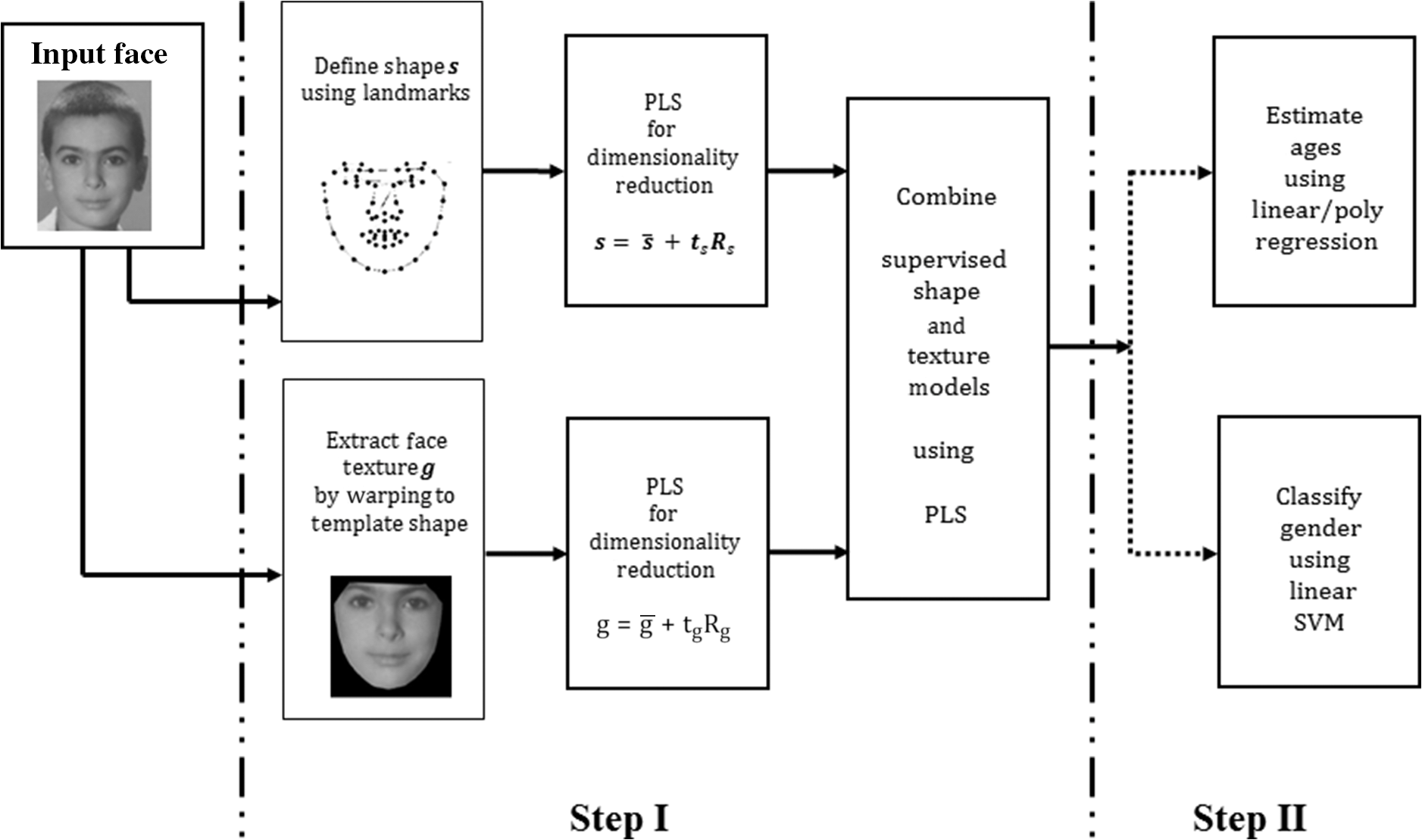
3. Related Algorithm to the Proposed Framework

3.1.

Partial Least-Squares for Dimension Reduction

PLS regression, introduced by Wold in Ref. 56, is a statistical method that creates latent features via a linear combination of the predictor ( $X$ ) and response ( $Y$ ) variables. It generalizes and combines features from multiple regression and PCA.⁵⁷ Hence, PLS has the ability to do both dimensionality reduction and regression simultaneously. The technique is very useful when there is need to predict a dependent variable from a large set of predictors. Although similar to PCA, it is much more powerful in regression applications, because PCA finds the direction of highest variance only in $X$ , so the principal components (PCs) best describe $X$ . However nothing guarantees that these PCs, which explain $X$ optimally, will be appropriate predictors of $Y$ . On the other hand, PLS searches for components (latent vectors) that capture directions of highest variance in $X$ as well as the direction that best relates $X$ and $Y$ (i.e., covariance between $X$ and $Y$ ). Hence it performs simultaneous decomposition of $X$ and $Y$ . In other words, PCA performs dimensionality reduction in an unsupervised manner, while PLS does in a supervised manner.

Let $X_{o} \in R^{N}$ denote an $n \times N$ matrix of predictor variables, where $n$ is the number of data samples and $N$ the dimensions (features) of the each data, and $Y_{o}$ be an $n \times M$ matrix of response variables. Here, $M$ refers to the response variable’s number of features, for most classification problems, $M = 1$ . PLS decomposes the two centered matrices (having zero mean) into

Eq. (1)

X_{o} = T P^{T} + E, Y_{o} = U Q^{T} + F,

where

T

and

U

are

n \times k

matrices of

k

extracted linear latent vectors also known as the latent scores, the matrices

P

and

Q

are loadings having

N \times k

and

M \times k

dimensions, respectively, the

n \times N

matrix

E

and the

n \times M

matrix

F

are the matrices of residuals. The scores

T

can be computed directly from the mean centered feature set

X_{o}

Eq. (2)

T = X_{o} W, X_{o} = X - \bar{X},

where

X

is the matrix of raw uncentered predictor variables,

\bar{X}

a matrix representing the mean of

X

has the same dimension with the zero-mean-predictor variable

X_{o}

, similarly, the matrices

Y

and

\bar{Y}

having the same dimension as

Y_{o}

represent the uncentered and mean response variables, respectively. The matrix of weights

W = {w_{1}, w_{2}, \dots w_{k}}

is computed by solving an optimization problem. The estimate of

k

’th direction vector is formulated as

Eq. (3)

{\hat{w}}_{k} = {argmax}_{r} X_{o}^{T} Y Y^{T} X_{o} w such that w^{T} w = 1 and X_{o}^{T} X_{o} w_{i} = 0,

for

i = 1 \dots k - 1

.

From Eq. (2), it is also possible to reconstruct the original data from the latent score by inverting the matrix $W$ . This operation is straightforward when $W$ is a square matrix, however only the approximate inverse can be computed for a nonsquare $W$ . However, only the approximate inverse can be computed for a nonsquare $W$

Eq. (4)

X_{o} = T R, R = W^{- 1} or R = W^{†} .

Here, we term

R

the projection coefficient.

Several methods for computing PLS have been proposed in the literature. In this work, we shall use the SIMPLS algorithm proposed by De Jong,⁵⁸ thereby taking advantage of the method’s speed.

Suppose we have a mean centered training set $X_{tr}$ consisting of observations, whose class labels are known and denoted by $Y_{tr}$ . Given a test set $X_{ts}$ , whose class label has to be predicted, PLS can be used for dimensionality reduction by projecting the test data onto the weight matrix $W$ . Hence, the latent scores matrix $T_{ts}$ for the test data is computed as shown below

Eq. (5)

T_{tr} = X_{tr} W, T_{ts} = X_{ts} W .

4. Proposed Framework

4.1.

Overview

Figure 1 illustrates the framework for age and gender classification. Step I describes the modeling of an sAM, which involves capturing shape and texture variations via PLS regression. The model is fully described in Sec. 4.2. Step II of the framework shows how the extracted facial features are utilized for age estimation or gender classification; this is outlined in Sec. 4.3. In Sec. 4.4, an algorithm summarizing the proposed framework is presented.

Fig. 1

sAM age and gender classification framework.

4.2.

Supervised Appearance Model

Like the conventional AAM, the proposed sAM captures both shape and texture variability from the training dataset. This is done by forming a parameterized model using PLS dimensionality reduction to capture the variations as well as combine them in a single model.

The shape of each face in the training DB is represented by a set of 2-D landmarks stacked to form a vector $s$ given by

Eq. (6)

s = {(x_{1}, x_{2}, \dots x_{n}, y_{1}, y_{2}, \dots y_{n})}^{T} .

As suggested by Cootes et al.,¹⁵ we remove rotational, translational, and scaling variations from the landmark locations by aligning all the shapes using generalized procrustes analysis.⁵⁹ Next, a supervised shape model is formed by performing PLS as described in Sec. 3. Here, we use the matrix of shapes

S = {s_{i}}

. as the predictor variable and the class labels are stored in a vector

Y

. Using Eq. (4), each shape can be represented using a linear equation

Eq. (7)

s - \bar{s} = t_{s} R_{s} .

This can be written as

Eq. (8)

s = \bar{s} + t_{s} R_{s},

where

\bar{s}

is the mean shape,

t_{s}

is a vector of latent scores representing the shapes, and

R_{s}

is the projection coefficient of shapes.

To build the supervised texture model, all face images are affine warped to the mean shape $\bar{s}$ ; this is done so that the control points of the training images match that of a fixed shape. Illumination variations are then normalized by applying a scaling and an offset to the warped images.¹⁵ Finally, each matrix of image pixel intensities (textures) is converted to vector $g$ . By applying PLS to the matrix $G = {g_{i}}$ , a linear model of textures is obtained

Eq. (9)

g = \bar{g} + t_{g} R_{g},

where

\bar{g}

is the gray-level texture,

t_{g}

is a vector of latent scores representing the texture, and

R_{g}

is the projection coefficient of textures.

Hence, both shape and texture can be summarized by the latent vectors $t_{s}$ and $t_{g}$ . Consequently, a combined model of shape and texture can be formed by concatenating the two vectors

Eq. (10)

t_{c} = (\begin{matrix} t_{s} & t_{g} \end{matrix}) .

To further eliminate the correlation that may exist between shape and texture, PLS is applied to

t_{c}

. Since both

t_{s}

and

t_{g}

have zero mean,

t_{c}

also has zero mean. Hence, the PLS decomposition can be achieved by directly substituting

t_{c}

into Eq. (4), where

t_{c}

replaces

X_{o}

, here, we use a matrix

L = {l_{1}, l_{2}, \dots l_{n}}

to represent the latent scores for all the faces in the DB.

Thus, the sAM describing each face can be represented by a linear equation

Eq. (11)

t_{c} = l P_{c}, P_{c} = (\begin{matrix} P_{s} & P_{g} \end{matrix}),

where

l

is a vector of latent scores representing both shape and texture of a particular individual and

P_{c}

is the projection coefficient of the combined model. It is worth noting that

P_{c}

has two components as shown in Eq. (11),

P_{s}

a projection coefficient associated with

t_{s}

and

P_{g}

which is associated with

t_{g}

.

Similar to the conventional AAM, the linear nature of the supervised model makes it possible to express both shape and texture in terms of the $l$

Eq. (12)

s = \bar{s} + l P_{s} R_{s}, g = \bar{g} + l P_{g} R_{g} .

We have now defined an sAM an extension of the AAM model, since the parameter $l$ summarizes both shape and texture information, it gives us a convenient way of representing faces with a view for solving the problems of age and gender classification.

4.3.

Age and Gender Classification

The sAM model contains both shape and texture components and can be supervised to model age and gender directly, which make it ideal as a facial model in these applications. In this work, we learn the aging pattern using a regression approach. Hence, an aging function relating faces to ages can be defined using

Eq. (13)

age = f (L),

where

age

is a vector of ages of all individuals in the DB,

L = {l_{1}, l_{2}, \dots l_{n}}

is a matrix for the sAM parameter for each face in the DB, and

n

is the total number of samples.

While several linear and nonlinear regressors have been used in the literature, here we experiment with simple models, hence we choose ordinary least-square (OLS) and QF regressions. Thus, for each face the $age$ is computed from its corresponding sAM parameter $l$ using

Eq. (14)

age = α + β^{T} l,

Eq. (15)

age = α + β_{1}^{T} l + β_{2}^{T} l^{2},

where

α

is the intercept also called an offset,

β_{1}

and

β_{2}

are vectors of regression coefficients, and Eqs. (14) and (15) correspond to OLS and QF, respectively.

Gender determination is a binary classification problem, where the test data are either labeled male or female. Given a training set $(x_{i}, y_{i})$ for $i = 1 \dots n$ , with $x_{i} \in R^{N}$ and $y_{i} \in {- 1, + 1}$ , a classifier is learned such that

Eq. (16)

f (x_{i}) {\begin{matrix} \geq 0 & y_{i} = + 1 \\ < 0 & y_{i} = - 1 \end{matrix} .

Here, we denote

+ 1

as male and

- 1

as female. While many classifiers have been proposed in the literature, SVM has been one of the most successful for binary classifications.

The goal of SVM is to find an optimal separating hyperplane (OSH) that best separates the two classes. It works by first mapping the training sample via a function $φ$ into a higher (infinite) dimensional space $F$ . Then, an OSH is found in $F$ by solving an optimization problem. However, the mapping from input space $X$ to the feature space $F$ is not done explicitly; rather, it is done via the kernel trick, which computes the inner dot products of the training data. For detailed explanation of SVM, the reader is referred to Ref. 60. In this work, the kernel function deployed is the linear kernel given by

Eq. (17)

K (x_{i}, x_{j}) = x_{i}^{T} x_{j} .

4.4.

Algorithm for the Proposed Framework

The proposed framework entails capturing the facial shape and texture using PLS regression, before combining the two statistical models into a single holistic model. We term this computational abstraction as sAM. Furthermore, the framework shows how the sAM parameterized face is used for age and gender classifications; this is summarized in Algorithm 1.

Algorithm 1

sAM age and gender classification framework.

1. Given a DB of face images, first train the sAM.

i. Describe the face shape by extracting 2-D landmarks of each face and stacking the

x

- and

y

-coordinates as a single vector using Eq. (6).

ii. Form shape-free patches by warping grayscale images to the mean shape and squeeze the face-image matrix into a long vector (

[340 \times 340] \times 1

).

iii. Utilize PLS to build the supervised shape and texture models, by employing Eqs. (8) and (9), respectively.

iv. Concatenate the shape and texture parameters (

t_{s}

and

t_{g}

) that were computed in iii, to form a combined model of appearance as expressed in Eq. (10).

v. Perform another PLS regression on

t_{c}

obtained in iv, to reduce dimensionality and to eliminate correlations that may exist between the shape and texture. Hence, the latent score

l

derived in Eq. (11) acts as a single parameter, which describes both shape and texture of a single face.

2. After training, the parameterized sAM variable

l

is used as the feature (predictor variable) to describe the face of an individual; consequently, this is then fed into the age or gender classifier.

i. For age estimation, linear or polynomial regressions are used.

ii. To achieve gender classification, use linear SVM.

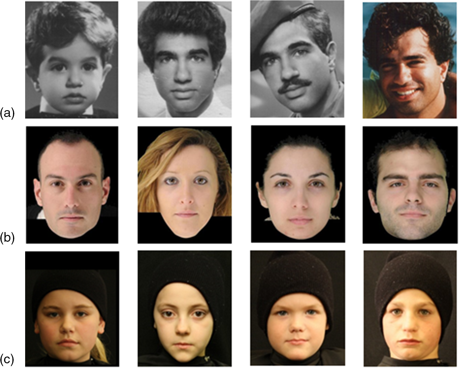
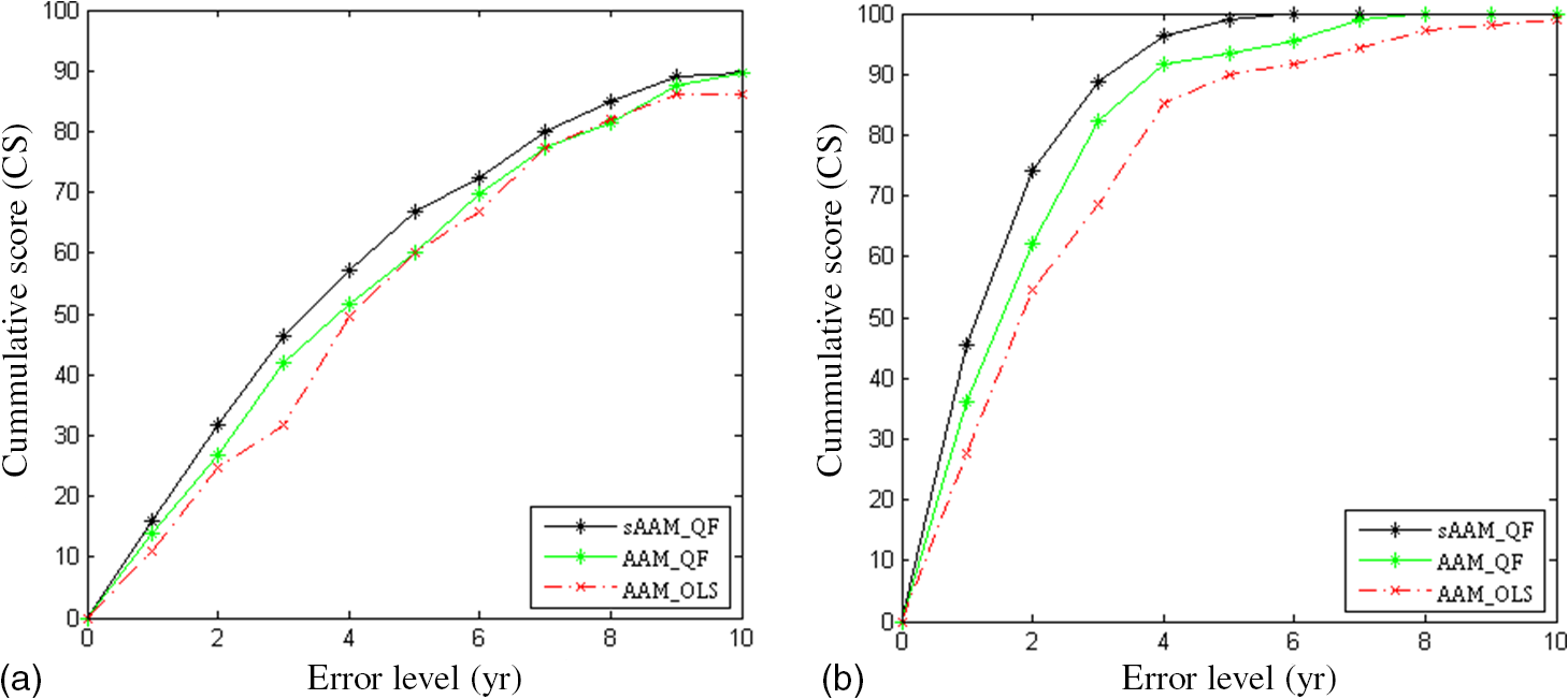
5. Experiments

In this section, the effectiveness of the proposed feature extraction technique is evaluated. sAM is compared to the conventional AAM in the two problems of age estimation and gender classification. Age estimation is evaluated by incorporating the sAM features into two simple traditional regression algorithms: linear and QFs. Furthermore, we perform gender classification by feeding the sAM features into a linear SVM classifier. Here, we have restricted our experiments to simple classifiers to fully explore the efficacy of the feature extraction method.

5.1.

Databases Used

Age estimation experiments are performed on one of the most widely used FGNET aging DB.⁶¹ Initially, gender classification experiments are conducted on the FGNET-AD, then to further show how age variation affects performance of gender classifiers, we perform two more experiments: one on Politecnico di Torino’s “HQFaces” DB⁶² and the other on the Dartmouth children’s faces DB.⁶³ In addition to comparing sAM to AAM, the algorithms are also compared to state-of-the-art work.

5.1.1.

FGNET-AD

The FGNET aging DB is made of 1002 images of 82 subjects, with ages distributed in the range of 0 to 69. Hence, each subject has multiple images. With more than 700 images within the age of 0 to 20, the age distribution is not balanced; this makes the FGNET-AD a challenging dataset. Additionally, the quality of the images varies from grayscale to colored, with individuals from different races displaying varying pose and facial expressions. Other inter- and intraquality variations include illumination, sharpness, and resolution. Gender distribution for FGNET-AD is 48 males and 34 females having 571 and 431 photographs, respectively.

5.1.2.

HQFaces database

HQFaces is a DB of 184 high-quality, controlled images collected at the Politecnico di Torino, Italy. All having a resolution of $4256 \times 2832$ and photographed under the same lightening conditions. The subjects are Caucasian, and predominantly adults having an age range of 13 to 50 yr, out of which 57% are male. For the purpose of our experiments, 143 frontal images were used.

5.1.3.

Dartmouth children’s faces database

Dartmouth children’s faces DB is an image library formed at the University of Dartmouth, Hanover, New Hampshire. It is made of high-quality images of 80 Caucasian children ranging from the ages of 6 to 16 yr, with a gender ratio of $50 / 50$ . Additionally, all subjects were photographed under two lightening conditions, at five angles and displaying eight facial expressions.

A sample of images contained in the above mentioned DBs is shown in Fig. 2. In this work, images from these sources were cropped to $340 \times 340 pixels$ ; this was done to reduce computational cost.

Fig. 2

Example of faces from the DBs used: (a) FGNET-AD, (b) HQFaces, and (c) Dartmouth faces.

5.2.

Age and Gender Classification Experiments

Face shape for the FGNET dataset is represented by a set of 68 landmarks defined in 2-D space $R^{2}$ . On the other two datasets, 79 fiducial points are used to describe the face shape. As stated earlier, for each face shape, the 2-D coordinates are converted into a single vector by stacking the $x$ -coordinates over the $y$ -coordinates as shown in Eq. (6).

Facial texture in the form of image pixels is captured by the approach of Cootes et al.¹⁵ First, all color images are converted to grayscale, then all the images are aligned to a mean shape via warping, thus “shape-free patches” are created using piecewise affine method,⁶⁴ a simple nonparametric warping technique that performs well on local distortions. Afterward, illumination normalization is conducted as stated earlier. Finally, each $340 \times 340$ image matrix is converted to a long ( $[340 \times 340] \times 1$ ) vector $g$ described in Eq. (9).

Using Eqs. (8) and (9), we compute the latent parameters of shape $t_{s}$ and texture $t_{g}$ , each of these two is represented using just eight components. Then, the second PLS is performed on an $(n \times 16)$ matrix. Considering the FGNET-AD, $n = 1002$ . Finally, the sAM parameter $l$ is represented by 13 components. We chose the number of components via cross validation.

To achieve age estimation, we implemented two regression algorithms as described earlier. In our experiment, the QF is computed in a sparse manner; as a form of regularization, we limited the number of observed powers. Hence, instead of computing the second-order terms of all 13 components, only the second-order terms of the first seven independent variables $(l_{1}^{2}, l_{2}^{2}, \dots l_{7}^{2})$ were used.

For age estimation, the vector $Y$ representing class labels contained individual ages of the training data, while in gender classification $+ 1$ and $- 1$ represented male and female genders, respectively.

To evaluate the accuracy of both age estimation and gender classification, we employed the leave-one-person-out (LOPO) cross-validation method. Here, the image of one person is used as the test set, and an estimator/classifier is trained using images of the remaining subjects. So, by the end of 82-folds, each subject in the FGNET-AD will have been used for testing. This approach mimics a real-life scenario, where the classifier is tested on an image that has not been seen before. In addition, the LOPO approach, unlike other cross-validation techniques, ensures consistency of results and ease of comparative evaluation of different algorithms.

The performance measures used for age estimation are mean absolute error (MAE) and cumulative score (CS), given by

Eq. (18)

MAE = \sum_{i = 1}^{N_{n}} | a g - a g^{'} | / N_{n},

Eq. (19)

CS (h) = N_{error \leq h} / N_{n} \times 100 %,

where

a g

is the ground truth age,

a g^{'}

is the estimated age,

N_{n}

is the number of test images, and

N_{error \leq h}

denotes the number of images on which the system makes absolute error not higher than

h

yr.

Gender classification performance is evaluated by detection rate (DR) also known as sensitivity. This is given by

Eq. (20)

DR = \sum True detections / \sum True samples \times 100 % .

First, we conducted an experiment on FGNET-AD, where we compared the results of sAM estimation and classification to those obtained using the conventional AAM and other state-of-the-art feature extraction techniques. A summary of our initial experiments on FGNET-AD is presented in Tables 2, 3, and Fig. 3.

Table 2

MAE for state-of-the-art age estimation algorithms on FGNET-AD (LOPO).

Feature	Algorithm	MAE	CS<10 (%)
AAM	WAS³⁰	8.06	$\approx 77$
AAM	QF¹⁷	7.57	$\approx 78$
AAM	SVM³¹	7.25	$\approx 76$
AAM	AGES³¹	6.77	$\approx 81$
AAM	AGES LDA³¹	6.22	$\approx 82$
AAM	RUN1⁶⁵	5.78	$\approx 84$
AAM	MLP³⁰	10.39	$\approx 60$
AAM	IIS-LLD⁶⁶	5.77	NA
AAM	OLS⁴¹	10.01	55.88
Proposed	sAM OLS	5.92	83.03
Proposed	sAM QF	5.49	85.34

Table 3

DR for gender classification algorithms on FGNET-AD (LOPO).

Feature	Algorithm	DR (%)
AAM	SVM¹⁸	72.95
AAM	Random forest⁶⁷	73.45
LPP	Sequential selection⁶⁷	72.26
LBP	SVM¹⁸	58.38
MLBP	SVM	62.77
Proposed	sAM SVM	76.65

Fig. 3

CSs of age estimation algorithms on FGNET.

Results show the superiority of the proposed sAM in age estimation and gender classification on a challenging benchmark DB. As shown in Table 2, the sAMs with linear and quadratic fits achieved 5.92 and 5.49 MAEs, respectively, using the LOPO cross-validation technique. Figure 3 shows CSs of algorithms at error levels between 0 and 10 yr. This demonstrates that sAM with quadratic fit has the most accurate estimation at all error levels with over 85% of the test data achieving estimation error below 10 yr. It is worth noting that the sAM based methods also have superior dimensionality reduction capability: while the number of AAM parameters used in most of the literature ranges from 50 to 200, using the sAM methods we were able to compress hundreds of appearance components into only eight variables. The gender classification experiment on the FGNET-AD shown in Table 3, also shows sAM with linear SVM classification achieved the best result with 76.65% DR. Other implementations of the AAM and LBP attained lower DRs.

To further evaluate the performance of the proposed framework, three additional experiments were conducted. We compared the performance of the better of our two age estimation implementations, i.e., sAM QF on the two controlled color image DBs (HQFaces and Dartmouth DB). As can be seen in Fig. 4, the CSs for error levels between 0 and 10 yr show that “sAM QF” is evidently better than the two AAM implementations. It is also not surprising that we achieved lower MAEs as compared to the result we attained on FGNET-AD. The reason behind 4.88 and 1.39 MAEs (as shown in Tables 4 and 5) on HQFaces and Dartmouth DB, respectively, was primarily due to the quality of the images. This shows that sAM, such as other feature extraction techniques, performs better under controlled conditions. The fact that the algorithm achieves the lowest estimation error on the Dartmouth DB implies that age discrimination is more apparent in children.

Table 4

MAE comparison on HQFaces DB (LOPO).

Feature	Algorithm	MAE	CS<10 (%)
AAM	QF¹⁷	5.12	$\approx 89$
AAM	OLS⁴¹	5.40	$\approx 86$
Proposed	sAM QF	4.88	$\approx 90$

Table 5

MAE comparison on Dartmouth DB (LOPO).

Feature	Algorithm	MAE	CS<10 (%)
AAM	QF¹⁷	1.87	$\approx 100$
AAM	OLS⁴¹	2.48	$\approx 96$
Proposed	sAM QF	1.39	100

Fig. 4

CSs for error levels from 0 to 10 yr: (a) HQFaces DB and (b) Dartmouth DB.

Next, experiments were conducted to assess the performance of our gender classification algorithm. Initially, we tested it in a holistic manner on the three DBs, as shown in Table 6, we achieved the best DR on HQFaces DB. Since HQFaces is made of predominantly adult faces, the result proves that gender discrimination is more evident in adults; consequently the classifier performs worst on children’s only DB (i.e., the Dartmouth DB). To further analyze this evidence, each image DB was split into seven age groups, 0 to 10, 11 to 20, 21 to 30, 31 to 40, 41 to 50, 51 to 60, and 61 to 70. The results presented in Table 7 depict two things: first, best DRs are achieved in the 21 to 30 age group, and second, it has been observed that the worst recorded result was on FGNET-AD’s 61 to 70 age group. This is obviously due to the size of the training data; as shown in Table 7, only seven images were used to train the algorithm at that instance. We therefore presume that sAM being a data-driven algorithm requires a sufficient amount of training data to achieve excellent classification results. If we were to sideline age groups with insufficient training data, it is then obvious that the performance of the gender classification for children’s faces (0 to 10 age group) remains clearly below what was achieved on adult faces where we had a sufficient number of training images.

Table 6

Gender classification DR on different DBs.

DB	DR (%)
HQFaces DB	92.50
Dartmouth DB	75.70
FGNET-AD	76.65

Table 7

Gender classification DR according to age groups.

Range	Dartmouth (%)	Images	HQFaces (%)	Images	FGNET-AD (%)	Images
0 to 10	68.98	53	—	—	63.99	411
11 to 20	88.89	27	95.00	60	84.01	319
21 to 30	—	—	95.29	85	91.61	143
31 to 40	—	–	70.00	10	86.96	69
41 to 50	—	—	60.00	5	87.18	39
51 to 60	—	—	—	—	71.42	14
61 to 70	—	—	—	—	42.86	7

6. Conclusion

We have proposed an sAM, which improves on the traditional AAM. When used for facial feature extraction, the model describes the face with very few components. For instance, we used just 13 components to effectively represent the face on FGNET-AD as opposed to AAM, which requires between 50 and 200 parameters. When used for age estimation, we achieved 5.49 MAE, which is comparable to most state-of-the-art algorithms and better than most algorithms that used AAM for feature extraction. Additionally, when used for gender classification, sAM outperforms most state-of-the-art work. This further proves the predict power and superior dimensionality reduction ability of the sAM. In the future, we hope to investigate the ability to reconstruct the human face using sAM with a view for conducting automatic facial age synthesis.

References

1.

G. Guo et al., “A study on automatic age estimation using a large database,” in 2009 IEEE 12th Int. Conf. on Computer Vision, 1986 –1991 (2009). http://dx.doi.org/10.1109/ICCV.2009.5459438 Google Scholar

2.

C.-B. Ng, Y.-H. Tay and B.-M. Goi, “A review of facial gender recognition,” Pattern Anal. Appl., 18 (4), 739 –755 (2015). http://dx.doi.org/10.1007/s10044-015-0499-6 Google Scholar

3.

E. Eidinger, R. Enbar and T. Hassner, “Age and gender estimation of unfiltered faces,” IEEE Trans. Inf. Forensics Secur., 9 (12), 2170 –2179 (2014). http://dx.doi.org/10.1109/TIFS.2014.2359646 Google Scholar

4.

G. Guo and G. Mu, “Simultaneous dimensionality reduction and human age estimation via kernel partial least squares regression,” in 2011 IEEE Conf. on Computer Vision and Pattern Recognition, 657 –664 (2011). http://dx.doi.org/10.1109/CVPR.2011.5995404 Google Scholar

5.

G. Levi and T. Hassner, “Age and gender classification using convolutional neural networks,” in 2015 IEEE Conf. on Computer Vision and Pattern Recognition Workshops (CVPRW ‘15), 34 –42 (2015). http://dx.doi.org/10.1109/CVPRW.2015.7301352 Google Scholar

6.

F. Metze et al., “Comparison of four approaches to age and gender recognition for telephone applications,” in IEEE Int. Conf. on Acoustics, Speech and Signal Processing (ICASSP ‘07), IV–1089 –IV–1092 (2007). http://dx.doi.org/10.1109/ICASSP.2007.367263 Google Scholar

7.

M. Li, K. J. Han and S. Narayanan, “Automatic speaker age and gender recognition using acoustic and prosodic level information fusion,” Comput. Speech Lang., 27 (1), 151 –167 (2013). http://dx.doi.org/10.1016/j.csl.2012.01.008 Google Scholar

8.

F. Burkhardt et al., “A database of age and gender annotated telephone speech,” in Proc. of the Seventh Int. Conf. on Language Resources and Evaluation (LREC ‘10), (2010). Google Scholar

9.

Y. Fu, G. Guo and T. Huang, “Age synthesis and estimation via faces: a survey,” IEEE Trans. Pattern Anal. Mach. Intell., 32 (11), 1955 –1976 (2010). http://dx.doi.org/10.1109/TPAMI.2010.36 ITPIDJ 0162-8828 Google Scholar

10.

G. Panis et al., “Overview of research on facial ageing using the FG-NET ageing database,” IET Biom., 5 (2), 37 –46 (2015). http://dx.doi.org/10.1049/iet-bmt.2014.0053 Google Scholar

11.

V. Bruce et al., “Sex discrimination: how do we tell the difference between male and female faces?,” Perception, 22 (2), 131 –152 (1993). http://dx.doi.org/10.1068/p220131 PCTNBA 0301-0066 Google Scholar

12.

H. A. Wild et al., “Recognition and sex categorization of adults’ and children’s faces: examining performance in the absence of sex-stereotyped cues,” J. Exp. Child Psychol., 77 (4), 269 –291 (2000). http://dx.doi.org/10.1006/jecp.1999.2554 JECPAE 0022-0965 Google Scholar

13.

C. Chen et al., “Face age estimation using model selection,” in 2010 IEEE Computer Society Conf. on Computer Vision Pattern Recognition—Workshops, 93 –99 (2010). http://dx.doi.org/10.1109/CVPRW.2010.5543820 Google Scholar

14.

G. Guo et al., “Human age estimation using bio-inspired features,” in IEEE Conf. on Computer Vision and Pattern Recognition (CVPR ’09), 112 –119 (2009). http://dx.doi.org/10.1109/CVPR.2009.5206681 Google Scholar

15.

T. F. Cootes, G. J. Edwards and C. J. Taylor, “Active appearance models,” in Computer Vision—(ECCV ’98), 484 –498 (1998). Google Scholar

16.

W. Chao, J. Liu and J. Ding, “Facial age estimation based on label-sensitive learning and age-oriented regression,” Pattern Recognit., 46 (3), 628 –641 (2013). http://dx.doi.org/10.1016/j.patcog.2012.09.011 Google Scholar

17.

A. Lanitis, C. Taylor and T. Cootes, “Toward automatic simulation of aging effects on face images,” IEEE Trans. Pattern Anal. Mach. Intell., 24 (4), 442 –455 (2002). http://dx.doi.org/10.1109/34.993553 ITPIDJ 0162-8828 Google Scholar

18.

W. Yang et al., “Gender classification via global-local features fusion,” Lect. Notes Comput. Sci., 7098 214 –220 (2011). http://dx.doi.org/10.1007/978-3-642-25449-9 LNCSD9 0302-9743 Google Scholar

19.

Y. H. Kwon and V. Lobo, “Age classification from facial images,” in Proc. IEEE Conf. Computer Vision Pattern Recognition (CVPR ‘94), 762 –767 (1994). http://dx.doi.org/10.1109/CVPR.1994.323894 Google Scholar

20.

W. B. Horng, C. P. Lee and C. W. Chen, “Classification of age groups based on facial features,” Tamkang J. Sci. Eng., 4 (3), 183 –192 (2001). http://dx.doi.org/10.6180/jase.2001.4.3.05 Google Scholar

21.

S. E. Choi et al., “Age estimation using a hierarchical classifier based on global and local facial features,” Pattern Recognit., 44 (6), 1262 –1281 (2011). http://dx.doi.org/10.1016/j.patcog.2010.12.005 Google Scholar

22.

C. R. Babu, E. S. Reddy and B. P. Rao, “Age group classification of facial images using rank based edge texture unit (RETU),” Procedia Comput. Sci., 45 215 –225 (2015). http://dx.doi.org/10.1016/j.procs.2015.03.124 Google Scholar

23.

N. Ramanathan and R. Chellappa, “Modeling age progression in young faces,” in 2006 IEEE Computer Society Conf. on Computer Vision Pattern Recognition, 387 –394 (2006). http://dx.doi.org/10.1109/CVPR.2006.187 Google Scholar

24.

H. Takimoto et al., “Robust gender and age estimation under varying facial pose,” Electron. Commun. Jpn., 91 (7), 32 –40 (2008). http://dx.doi.org/10.1002/ecj.v91:7 Google Scholar

25.

Y. Fu, Y. Xu and T. S. Huang, “Estimating human age by manifold analysis of face pictures and regression on aging features,” in 2007 IEEE Int. Conf. on Multimedia and Expo, 1383 –1386 (2007). http://dx.doi.org/10.1109/ICME.2007.4284917 Google Scholar

26.

G. Guo et al., “Image-based human age estimation by manifold learning and locally adjusted robust regression,” IEEE Trans. Image Process., 17 (7), 1178 –1188 (2008). http://dx.doi.org/10.1109/TIP.2008.924280 IIPRE4 1057-7149 Google Scholar

27.

M. Riesenhuber and T. Poggio, “Hierarchical models of object recognition in cortex,” Nat. Neurosci., 2 (11), 1019 –1025 (1999). http://dx.doi.org/10.1038/14819 NANEFN 1097-6256 Google Scholar

28.

M. Y. El Dib and M. El-Saban, “Human age estimation using enhanced bio-inspired features (EBIF),” in 2010 IEEE Int. Conf. Image Processing, 1589 –1592 (2010). http://dx.doi.org/10.1109/ICIP.2010.5651440 Google Scholar

29.

T. Wu, P. Turaga and R. Chellappa, “Age estimation and face verification across aging,” IEEE Trans. Inf. Forensics Secur., 7 (6), 1780 –1788 (2012). http://dx.doi.org/10.1109/TIFS.2012.2213812 Google Scholar

30.

A. Lanitis, C. Draganova and C. Christodoulou, “Comparing different classifiers for automatic age estimation,” IEEE Trans. Syst. Man Cybern. B, 34 (1), 621 –628 (2004). http://dx.doi.org/10.1109/TSMCB.2003.817091 Google Scholar

31.

X. Geng, Z.-H. Zhou and K. Smith-Miles, “Automatic age estimation based on facial aging patterns,” IEEE Trans. Pattern Anal. Mach. Intell., 29 (12), 2234 –2240 (2007). http://dx.doi.org/10.1109/TPAMI.2007.70733 Google Scholar

32.

S. Yan et al., “Regression from patch-kernel,” in IEEE Conf. on Computer Vision and Pattern Recognition (CVPR ’08), 1 –8 (2008). http://dx.doi.org/10.1109/CVPR.2008.4587405 Google Scholar

33.

C. Fernández, I. Huerta and A. Prati, “A comparative evaluation of regression learning algorithms for facial age estimation,” in FFER Conjunction with ICPR, (2014). Google Scholar

34.

V. F. Ferrario et al., “Sexual dimorphism in the human face assessed by Euclidean distance matrix analysis,” J. Anat., 183 (Pt 3), 593 (1993). JOANAY 0021-8782 Google Scholar

35.

A. M. Burton, V. Bruce and N. Dench, “What’s the difference between men and women? Evidence from facial measurement,” Perception, 22 (2), 153 –176 (1993). http://dx.doi.org/10.1068/p220153 PCTNBA 0301-0066 Google Scholar

36.

J.-M. Fellous, “Gender discrimination and prediction on the basis of facial metric information,” Vision Res., 37 (14), 1961 –1973 (1997). http://dx.doi.org/10.1016/S0042-6989(97)00010-2 VISRAM 0042-6989 Google Scholar

37.

B. Moghaddam and M.-H. Yang, “Learning gender with support faces,” IEEE Trans. Pattern Anal. Mach. Intell., 24 (5), 707 –711 (2002). http://dx.doi.org/10.1109/34.1000244 Google Scholar

38.

G. Edwards, Learning to Identify Faces in Images and Video Sequences, (1999). Google Scholar

39.

M. C. Ionita, P. Corcoran and V. Buzuloiu, “On colour texture normalization for active appearance models,” IEEE Trans. Image Process., 18 (6), 1372 –1378 (2009). http://dx.doi.org/10.1109/TIP.2009.2017163 IIPRE4 1057-7149 Google Scholar

40.

Y.-I. Ohta, T. Kanade and T. Sakai, “Colour information for region segmentation,” Comput. Graphics Image Process., 13 (1), 222 –241 (1980). http://dx.doi.org/10.1016/0146-664X(80)90047-7 Google Scholar

41.

A. M. Bukar, H. Ugail and D. Connah, “Individualised model of facial age synthesis based on constrained regression,” in 2015 Int. Conf. on Image Processing Theory, Tools and Applications (IPTA ‘15), 285 –290 (2015). http://dx.doi.org/10.1109/IPTA.2015.7367147 Google Scholar

42.

Y. Sun, S. Chen and B. Yin, “Colour face recognition based on quaternion matrix representation,” Pattern Recognit. Lett., 32 (4), 597 –605 (2011). http://dx.doi.org/10.1016/j.patrec.2010.11.004 PRLEDG 0167-8655 Google Scholar

43.

B. Chen et al., “Colour image analysis by quaternion-type moments,” J. Math. Imaging Vision, 51 (1), 124 –144 (2015). http://dx.doi.org/10.1007/s10851-014-0511-6 Google Scholar

44.

L. Deng and D. Yu, “Deep learning: methods and applications,” Found. Trends^® Signal Process., 7 (3–4), 197 –387 (2013). http://dx.doi.org/10.1561/2000000039 Google Scholar

45.

C. Yan et al., “Age estimation based on convolutional neural network,” Advances in Multimedia Information Processing—PCM 2014, 211 –220 Springer-Verlag, New York (2014). Google Scholar

46.

Y. LeCun, Y. Bengio and G. Hinton, “Deep learning,” Nature, 521 (7553), 436 –444 (2015). http://dx.doi.org/10.1038/nature14539 Google Scholar

47.

D. Huang et al., “Local binary patterns and its application to facial image analysis: a survey,” IEEE Trans. Syst. Man Cybern. C, 41 (6), 765 –781 (2011). http://dx.doi.org/10.1109/TSMCC.2011.2118750 Google Scholar

48.

A. F. Abate et al., “2D and 3D face recognition: a survey,” Pattern Recognit. Lett., 28 (14), 1885 –1906 (2007). http://dx.doi.org/10.1016/j.patrec.2006.12.018 PRLEDG 0167-8655 Google Scholar

49.

L. Shen and L. Bai, “A review on Gabor wavelets for face recognition,” Pattern Anal. Appl., 9 (2–3), 273 –292 (2006). http://dx.doi.org/10.1007/s10044-006-0033-y Google Scholar

50.

X. Wen et al., “A rapid learning algorithm for vehicle classification,” Inf. Sci., 295 395 –406 (2015). http://dx.doi.org/10.1016/j.ins.2014.10.040 ISIJBC 0020-0255 Google Scholar

51.

P. Viola and M. Jones, “Rapid object detection using a boosted cascade of simple features,” in Proc. 2001 IEEE Computer Society Conf. on Computer Vision Pattern Recognition (CVPR ‘01), I–511 –I–518 (2001). http://dx.doi.org/10.1109/CVPR.2001.990517 Google Scholar

52.

B. Wu et al., “Fast rotation invariant multi-view face detection based on real adaboost,” in Proc. Sixth IEEE Int. Conf. on Automatic Face and Gesture Recognition, 79 –84 (2004). http://dx.doi.org/10.1109/AFGR.2004.1301512 Google Scholar

53.

G. Tzimiropoulos, S. Zafeiriou and M. Pantic, “Subspace learning from image gradient orientations,” IEEE Trans. Pattern Anal. Mach. Intell., 34 (12), 2454 –2466 (2012). http://dx.doi.org/10.1109/TPAMI.2012.40 Google Scholar

54.

X. Gao et al., “A review of active appearance models,” IEEE Trans. Syst. Man Cybern. C, 40 (2), 145 –158 (2010). http://dx.doi.org/10.1109/TSMCC.2009.2035631 Google Scholar

55.

J. Ngiam et al., “On optimization methods for deep learning,” in Int. Conf.on Machine Learning, 265 –272 (2011). Google Scholar

56.

H. Wold, “Estimation of principal components and related models by iterative least squares,” Multivariate Analysis, 391 –420 1966). Google Scholar

57.

H. Abdi, “Partial least squares regression and projection on latent structure regression (PLS Regression),” Wiley Interdiscip. Rev. Comput. Stat., 2 (1), 97 –106 (2010). http://dx.doi.org/10.1002/wics.51 Google Scholar

58.

S. De Jong, “SIMPLS: an alternative approach to partial least squares regression,” Chemom. Intell. Lab. Syst., 18 (3), 251 –263 (1993). http://dx.doi.org/10.1016/0169-7439(93)85002-X Google Scholar

59.

J. C. Gower, “Generalized procrustes analysis,” Psychometrika, 40 (1), 33 –51 (1975). http://dx.doi.org/10.1007/BF02291478 0033-3123 Google Scholar

60.

A. J. Smola and B. Schölkopf, “A tutorial on support vector regression,” Stat. Comput., 14 (3), 199 –222 (2004). http://dx.doi.org/10.1023/B:STCO.0000035301.49549.88 STACE3 0960-3174 Google Scholar

61.

FG-NET (Face and Gesture Recognition Network), “The Fg-Net aging database,” (2014) http://wwwprima.inrialpes.fr/FGnet/ ( September ). 2014). Google Scholar

62.

T. F. Vieira et al., “Detecting siblings in image pairs,” Visual Comput., 30 (12), 1333 –1345 (2014). http://dx.doi.org/10.1007/s00371-013-0884-3 VICOE5 0178-2789 Google Scholar

63.

K. A. Dalrymple, J. Gomez and B. Duchaine, “The Dartmouth database of children’s faces: acquisition and validation of a new face stimulus set,” PLoS One, 8 (11), e79131 (2013). http://dx.doi.org/10.1371/journal.pone.0079131 POLNCL 1932-6203 Google Scholar

64.

C. A. Glasbey and K. V. Mardia, “A review of image-warping methods,” J. Appl. Stat., 25 (2), 155 –171 (1998). http://dx.doi.org/10.1080/02664769823151 Google Scholar

65.

S. Yan et al., “Learning auto-structured regressor from uncertain nonnegative labels,” in 2007 IEEE 11th Int. Conf. on Computer Vision, 1 –8 (2007). http://dx.doi.org/10.1109/ICCV.2007.4409050 Google Scholar

66.

X. Geng, C. Yin and Z.-H. Zhou, “Facial age estimation by learning from label distributions,” IEEE Trans. Pattern Anal. Mach. Intell., 35 (10), 2401 –2412 (2013). http://dx.doi.org/10.1109/TPAMI.2013.51 Google Scholar

67.

Y. Wang et al., “Gender classification from infants to seniors,” in 2010 Fourth IEEE Int. Conf. on Biometrics: Theory Applications and Systems (BTAS ‘10), 1 –6 (2010). http://dx.doi.org/10.1109/BTAS.2010.5634518 Google Scholar

Biography

Ali Maina Bukar received his MSc degree from the School of Computing Science and Digital Media, Robert Gordon University, Aberdeen, UK, in 2010. He is currently working toward his PhD at the School of Media Design and Technology, University of Bradford, UK. His research interests include pattern recognition, machine learning, computer vision, and signal processing.

Hassan Ugail has received a first class BSc Honors degree in mathematics from King’s College London and PhD in the field of geometric design from the School of Mathematics, University of Leeds. He is the director of the Centre for Visual Computing at Bradford. His research interests include geometric and functional design and three-dimensional (3-D) imaging. He has a number of patents on techniques relating to geometry modeling, animation, and 3-D data exchange.

David Connah has a multidisciplinary background in biology (BSc), artificial intelligence (MSc), and digital imaging (PhD), and specializes in the role of color in digital imaging and computer vision applications, from both computational and perceptual perspectives. His research interests include multispectral imaging, image fusion, camera characterization, and human perception and performance. He has published over 25 journal and conference papers and is the holder of 3 patents in image processing.

CC BY: © The Authors. Published by SPIE under a Creative Commons Attribution 4.0 Unported License. Distribution or reproduction of this work in whole or in part requires full attribution of the original publication, including its DOI.

Citation Download Citation

Ali Maina Bukar, Hassan Ugail, and David Connah "Automatic age and gender classification using supervised appearance model," Journal of Electronic Imaging 25(6), 061605 (1 August 2016). https://doi.org/10.1117/1.JEI.25.6.061605

Published: 1 August 2016

Access the abstract

JOURNAL ARTICLE
11 PAGES

DOWNLOAD PAPER SAVE TO MY LIBRARY

GET CITATION

CITATIONS

Cited by 24 scholarly publications and 1 patent.

Explore citations on Lens.org

KEYWORDS

Feature extraction

Principal component analysis

Image classification

Binary data

Data modeling

Shape analysis

Statistical analysis

1.

Introduction

2.

Previous and Related Work

2.1.

Age Estimation

2.1.1.

Feature extraction

2.1.2.

Age learning

2.2.

Gender Classification

Table 1

3.

Related Algorithm to the Proposed Framework

3.1.

Partial Least-Squares for Dimension Reduction

Eq. (1)

Eq. (2)

Eq. (3)

Eq. (4)

Eq. (5)

4.

Proposed Framework

4.1.

Overview

Fig. 1

4.2.

Supervised Appearance Model

Eq. (6)

Eq. (7)

Eq. (8)

Eq. (9)

Eq. (10)

Eq. (11)

Eq. (12)

4.3.

Age and Gender Classification

Eq. (13)

Eq. (14)

Eq. (15)

Eq. (16)

Eq. (17)

4.4.

Algorithm for the Proposed Framework

Algorithm 1

5.

Experiments

5.1.

Databases Used

5.1.1.

FGNET-AD

5.1.2.

HQFaces database

5.1.3.

Dartmouth children’s faces database

Fig. 2

5.2.

Age and Gender Classification Experiments

Eq. (18)

Eq. (19)

Eq. (20)

Table 2

Table 3

Fig. 3

Table 4

Table 5

Fig. 4

Table 6

Table 7

6.

Conclusion

References

Biography

Show All Keywords

Keywords/Phrases

Search In:

Publication Years