1.

Introduction

With the development of communications, the security problem for confidential information has emerged. Also, there is theft or damage to data repositories to which there is no free access. Therefore, there have appeared several encryption procedures for information, in particular, images.¹ There are some new methods using the Hilbert transform,² chaos,³ the hyper-chaos,⁴ or even the advanced encryption standard (AES) cryptosystem⁵ with the CBC encryption mode,⁶ although this way is a sequential encryption. The first two are fast, but they have a robustness problem,⁶ in that it is not specifically mentioned what the number of elements in the key set is. The hyper-chaos method⁴ is a key size of $2^{167}$ and they only speak of brute force attacks and no other type of analysis, for example, differential⁷ and linear⁸ attacks. By the way, the AES cryptosystem has no problem with any of them yet.⁹ Moreover, the AES key set can reach $2^{256}$ elements. It is also important to note that the AES algorithm uses the substitution operation through a box. The substitution operation gives nonlinearity to the encryption process,¹⁰ and none of the aforementioned algorithms. In fact, the nonlinearity of the AES box is superior to data encryption standard (DES) and triple-DES boxes.¹¹ Also, there are encryptions for color images using the transformed Fourier,¹² the gyrator and Arnold transforms.¹³ However, in these two latest investigations, the specific algorithm complexity is not shown. On the other hand, there are some color image encryption investigations¹⁴ where they do not specify the set key size. Other optical papers^15–17 demonsrrate cipher images in an original way, but they do not clearly show the key set size. There is also an important paper in image encryption,¹⁸ although this alters the original image when it is decrypted, and this is important because in some countries it is not allowed. There is an interesting investigation using a chaotic map to encrypt images,¹⁹ but that paper does not employ a test of NIST Special Publication 800-22 to measure the randomness of the encrypted images.

We decided to use the AES algorithm for images encryption for the following reasons: it is a recent symmetric encryption system, and it is also the International Standard at this time.⁵ This makes the AES algorithm one of the most studied worldwide. However, an efficient method for breaking it has not yet been found.²⁰ The encryption “quality” of a figure concerns the randomness degree in the image bits distribution. Several methods have been utilized to measure the randomness degree.²¹ In this work, the following are used: correlation coefficients; horizontal, vertical, and diagonal,²² entropy and discrete Fourier transform (DFT). The latter measures the periodicity degree of the zeroes and ones string, i.e., whether or not a pattern is followed. Furthermore, a different way is proposed to measure the randomness degree of the encrypted figure bits using a “goodness-of-fit test.”²²

This investigation does not use compression on images because there are some countries whose security areas do not allow compression in the encryption image.²³ In other words, it does not utilize the process: compression–encryption → decryption–decompression. It is only employs encryption → decryption. Five images as prototypes to be encrypted are used, of which four are in most papers on encryption figures; these images are the following: baboon, Barbara, Lena, and peppers. A criterion to select the fifth figure to be encrypted is proposed. All the images have a different difficulty degree to be encrypted when a symmetric cryptosystem is used. This difficulty depends on the randomness degree of the figure bits to be encrypted, since an image with a high randomness degree in its bits distribution is easier to encrypt than a figure that has low randomness, when ECB encryption mode is used. This paper is organized as follows: this section presents a very synthetic state of art and Sec. 2 shows the basic concepts to be used in this investigation. The bijective function is addressed in Sec. 3, and is also demonstrated. Section 4 approaches the AES algorithm with variable permutations, and constructs a permutation in the whole image. Ways to measure the randomness degree are presented in Sec. 5. Section 6 shows the encrypted figures analysis with damage, and the outcome of the randomness degree in the encrypted figures is shown in Sec. 7. Section 8 discusses the results. Finally, the conclusions are given in Sec. 9.

2.

Preliminary Concept

Even though the AES algorithm is the most studied in the world, an efficient way to solve it is not known. Another important issue to clarify is that AES is a symmetric algorithm, which makes it a very fast method with which to encrypt data. However, if a figure with a low randomness degree in its bits distribution is encrypted using the AES algorithm without any modification, perhaps the image encrypted could provide information, i.e., the distribution of the different shades of basic colors follow a certain pattern. So, it is necessary to employ an additional element in the algorithm. Thus, this paper proposes applying a different permutation in each 128 bits block. This permutation is applied in the first round after the x-or operation. The reason why the permutation is not used at the first round entrance as is triple-DES¹¹ is because some images have areas with the same color, such as black or white. In this situation, whatever permutation applied to a zeroes or ones string would not make any change in the chain. If the permutation is used after the x-or operation, then it allows for changing some string bits. Another question is why in the first round? Well, it is understood that the information is mixed in each round, so any change carried out by the permutation at the first round will have more opportunity to mix the information. Therefore, at the end of the encryption process the zeroes and ones string will be random.

As is known, the transcendental numbers are not the solution for any polynomial whose form is $a_n{x}^n+a_{(n-1)}{x}^{(n-1)}+\dots +a_0$ with $a_i$ $ϵ$ $Z$, and besides, all the numbers after the decimal point have the property of not following any periodicity,²⁴ making them good candidates to be used as pseudorandom numbers.²⁵ In fact, for this feature, the irrational numbers are employed in Has-Sha functions.²⁶ The transcendent number used in this investigation is $pi$, because it has been studied for a long time.²⁷ On the other hand, the permutations generated depend on the AES key in accordance with the following procedure: denoted as $l$ the integer which represents the 128 bits chain AES key. Then the product $(pi)l$ is also a transcendental number. Thus, using this last number it is possible to get the constants to build the permutations.

The entropy is measured according to the formula: $-\sum _{x\epsilon X}{P}_r(x){\log }_2{P}_r(x)$. When working with each basic color of the images—red, green, or blue—each one can be described as 1 byte, i.e., 256 levels are sufficient for each. So, if each basic color has a uniform distribution, all points are equally likely, and the entropy value is 8.²⁸ This means the information is completely random. However, in practice, this is not so. Then values are sought as close to 8 as possible, in the basic colors’ distribution red, green, and blue of the encrypted figure. If the image is mono-colored, the procedure is basically the same, since only 1 byte is used to describe the gray color, i.e., 256 different gray levels, following the same reasoning as the color images.

A statistic test to evaluate the chain bits randomness is formulated by means of a null hypothesis $H_0$ versus an alternative $H_a$. The null hypothesis establishes that the bits sequence is random and the alternative hypothesis is the opposite. To accept or reject the null hypothesis, a statisticand a threshold are used. If the statistic based on the data has a value bigger than the threshold, it implies that the null hypothesis is accepted, otherwise $H_0$ is rejected. In any hypothesis test scheme there are two errors, namely, type I and type II errors. The type I error is committed when $H_0$ is rejected when this hypothesis is true and the type II error is committed when $H_0$ is accepted and it is false. The type I error can be controlled, because it is supposed that $H_0$ is the more important of the two hypotheses. The amount used in this research for type I error is $\alpha =0.01$, although the value $\alpha =0.001$ can be used.²¹ The error $\alpha$ is also called the significance level.

The probability distributions used in the randomness tests are: Chi-square ${\chi }^2$ and complementary error function $\mathrm{erfc}(z)=(2/\sqrt{pi})$ ${\int }_z^{\infty }{e}^{-u^2}\mathrm{d}u$.²⁹ It is possible to express the $\mathrm{erfc}(z)$ function in terms of a normal standard cumulative distribution according to the following reasoning:

The normal standard cumulative distribution, and

The next variable change is proposed for Eq. (2), $u=v/\sqrt{2}$ and $du=dv/\sqrt{2}$.

Therefore, $\mathrm{erfc}(z)=(2/\sqrt{pi}){\int }_{\sqrt{2}z}^{\infty }{e}^{-v^2/2}\mathrm{d}v$ then, this last expression is written thus: $\mathrm{erfc}(z=w/\sqrt{2})=2/\sqrt{2pi}({\int }_w^{\infty }{e}^{-v^2/2}\mathrm{d}v)$, thus

Regarding the concept of a real-time decision relates to the following: it is known that there are important decisions for which there is a short time to make them, therefore, the procedure expressed here contributes to the process of making a timely decision.

3.

Bijective Function

Let us have the following considerations: given a natural $m\ge 2$ the sets $N_m=\{n\epsilon N|0\le n\le m!-1\}$ and ${\mathrm{\Pi }}_m=\{\pi \}$ can be defined, such that $\pi$ is a permutation of the $0,1,\dots ,m-1$ array. According to the Euclid division algorithm,³⁰ $\forall$ $n\epsilon N_m$, this one can be written in a unique way as follows:

Note that for a given $m$, $(m-1)!,(m-2)!,\dots 1!,0!$ are fixed. It will be seen in the algorithm description that the constant $C_{m-1}=0$. Also, it is easy to prove that

When the constants $C_0,C_1\dots C_{m-2}$ are calculated, the following algorithm can be constructed:

The arrangement of positive integers $X[C_0],X[C_1]\dots X[C_{m-2}]$ and $X[C_{m-1}]$ is a permutation of the $\mathrm{0,1}\dots m-1$ array. This procedure is made in $m-1$ steps. Regarding the complexity to implement this algorithm is $O(m)$ because at every step a removal and replacement of an item is made. The remainder is unchanged.

Clearly, in the case of images with 250,000 pixel files or more the algorithm with a $O(m)$ complexity represents an important advantage. It is clear that the algorithm presented above defines a function that goes from $N_m$ to ${\mathrm{\Pi }}_m$; denoted as $I_m$. Next $I_m$: $N_m\to {\mathrm{\Pi }}_m$ is demonstrated as a bijective function.

4.

Advanced Encryption Standard with Variable Permutations

At this point, the way to use the algorithm presented above to construct a pseudorandom permutation over $m$ positions array and then how to apply this tool in image encryption is shown. In this vein, it proceeds as follows: If the algorithm developed in the previous section is observed, knowing the values $C_i$ for $i=0,1,\dots ,m-1$ a permutation can be constructed. Note that it is not important to know the $n$ number with all its digits, fortunately, because it is impossible to work with integers around $\mathrm{250,000}!-1$ or higher since they are huge.

In this sense, the quantities $(m-1)!$, $(m-2)!\dots$ are used only as marks, so it is not important to write all the digits. Then, the next question to address is how to choose pseudorandom values $C_i$ for $i=0,1,\dots m-1$. First, the permutations are built on 128 position arrangements using the $pi$ number thus:

For the whole image, the number of items to permute, $m$, can have 250,000 or more elements. For a situation like this, the procedure is the same as when $m=128$. There are some differences, namely, the size of the blocks in this case $a_i$ is 24 bits. This is because many of the current images do not exceed $2^{24}$ bits in the spatial resolution.

Clearly, these blocks also represent positive integers. So, the $C_i$ can be defined as $C_i=a_i$ mod. $m-i$, for $i=0,1,\dots ,m-2$ and $C_{m-1}=0$.

Sometimes, some bytes can be subtracted from the image to be encrypted according to the next criterion: if $24(m)$ mod. $128\not\equiv 0$ where $m$ is the pixels number of the image, then the minimum amount of bytes required is subtracted, say $n$, such that $24(m)-8(n)$ mod.$128\equiv 0$. It is important to point out that $8n<128$ and this number of bits, $8n$, is not encrypted. Once the values $C_0,C_1,\dots ,C_{m-2}$ are known, the ${\pi }_m$ permutations on $m$ elements array can be calculated according to the procedure described in Sec. 3. In the case of AES with variable permutations the constant sets that are necessary according to the image size are calculated.

In a particular situation such as: a secure communication scheme such as public key infrastructure (PKI),³¹ where the AES-128 and Elgamal³² cryptosystems are used, the procedure is as follows:

In this research, the signature and nonrepudiation as part of the structure of PKI secure communication are not mentioned³³ since they are not within the scope of this work.

Figures 1 and 2 flowcharts are shown; namely, the first illustrates how the permutation for the entire image is obtained. The second exemplifies how the variable permutations of 128 positions are developed.

Fig. 1

Permutation for the entire image. The $n$ is the number of pixels. The product $(l)*(\pi )$, where $l$ is the integer associated to the key. The $a(i)$ is the block number $i$ of 24 bits, after the decimal point of product $(l)*(\pi )$. The constant $c(i)$ is the number $i$ to obtain the permutation $Y(i)$. The $W(i)$ is the element number $i$ of the permuted image.

Fig. 2

Permutations of 128 positions in the cipher of the image. The $n$ is the number of blocks of 128 bits of the permutated image. The $a_j^{*}(i)$ is the byte number $i$ of the product $(l)*(\pi )$, after the decimal point. The $Z_j(i)$ is the bit of position $i$ of block $j$ of 128 bits to be ciphered. The $k_1$ is the first key of the schedule of keys. The $E_j$ is the block number $j$ of 128 bits ciphered. The $Z_j^{*}(i)$ is the result of the operation x-or between $Z_j$ and $k_1$. The $W_j$ is the block that results after the application of permutation $Y_j$.

Regarding the security of this cryptosystem, the following can be mentioned: the worst that can happen is that the AES key could be known, because if this encryption scheme is used, the permutation over the whole image and the variable permutations applied in each block can be calculated. So, in this situation, the maximum security is $2^{128}$. However, if we want to find the key, taking as a plaintext the permuted image using the brute force attack, then this could be a problem with a complexity of $2^{843}$; because in a previous work³⁴ a strong evidence was given that the DES algorithm with variable permutation has a complexity of $2^{56}\times (64!)$, where the Monte Carlo method was used. Clearly, if the problem is to find the key from the initial image, the solution to the problem would be more complex. Cases of plaintext are chosen as differential and linear attacks, which are not applicable to the AES cryptosystem due to the way the substitution box is constructed.⁶

5.

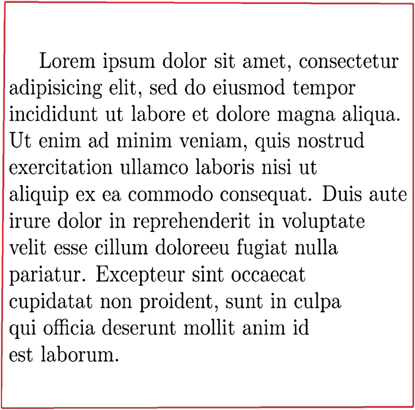
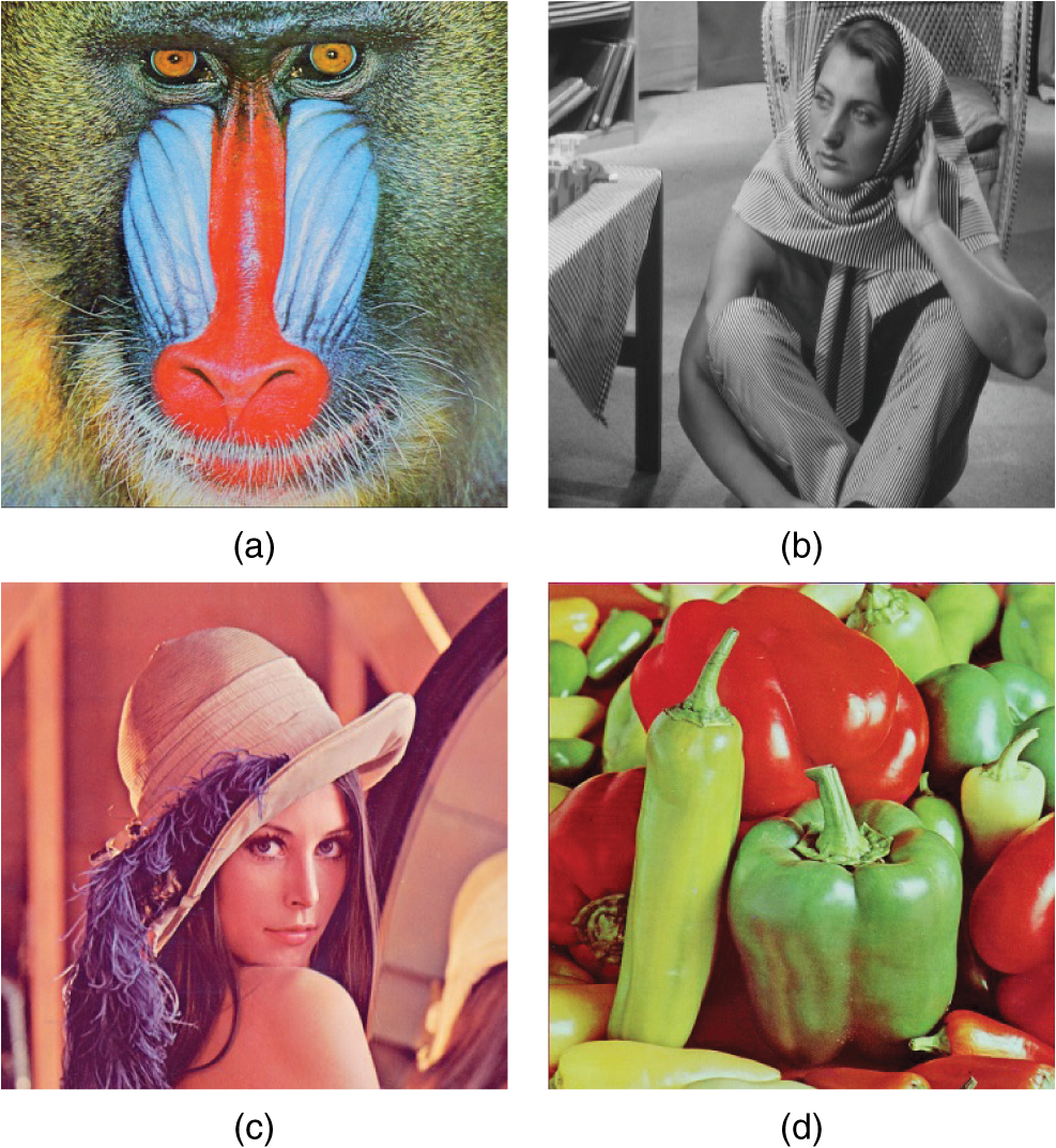
Randomness Analysis

5.3.

Criteria of Image Selection

In Sec. 1, it was mentioned that a criterion would be presented to choose a fifth figure to be encrypted. This criterion is based on a characteristic of the goodness-of-fit test that tells us the following: if the tone distribution in each basic color was completely random, then ${\chi }^2=0$. In fact, this means that the color histogram follows a uniform distribution. However, if ${\chi }^2$ has a large value for each basic color, it means they have a defined order. So the authors propose choosing an image that has a ${\chi }^2$ as large as possible for each primary color. In this paper, a figure with the values of ${\chi }^2$: ${\chi }_r^2=106361059.17$, ${\chi }_g^2=106647915.51$ and ${\chi }_b^2=107366956.56$, for the red, green, and blue colors, respectively, is proposed. This image is a simulation of Latin text that is usually used in graphic design typographic demonstrations or drafts.³⁸ This image is shown in Fig. 3.

Fig. 3

Type image to be encrypted.

On the other hand, there is another reason for making the ${\chi }^2$ very large since there are many images with relatively small values for each statistical ${\chi }^2$ of the basic color, say less than half a million; in these cases the AES cryptosystem can be applied directly, i.e., it is not necessary to use variable permutations to encrypt an image and the result passes the above tests and even the proposal. For example, image (b) of Fig. 6—Barbara—has the quantities of ${\chi }^2$ for the primary colors red, green, and blue: ${\chi }_r^2=95086.89$, ${\chi }_g^2=95086.89$, and ${\chi }_b^2=95086.89$; these values are equal because it is a mono-colored image. In Fig. 4, Barbara and her encrypted image are presented without using variable permutations. By the way, Fig. 4(a) is ciphered considering the same gray level of each pixel in the three planes and is later encrypted in blocks of 128 bits.

Fig. 4

Comparing the original (a) and encrypted (b) images without variable permutation.

For figures with a very large ${\chi }^2$ for each different basic color, say more than 100 million, the variable permutations must be applied so that the encryption process is effective. Figure 5 shows when the encryption process can be ineffective in a simple way, since the ${\chi }^2$ for the primary colors are: ${\chi }_r^2=5691872.24$, ${\chi }_g^2=5714519.25$, and ${\chi }_b^2=5706278.92$ for red, green, and blue, respectively. Remember, it was noted above that the rejection region threshold is 324.78 for $\alpha =0.001$ as maximum. Furthermore, the ${\chi }^2$ values mentioned above are much higher, in fact, about 6 million.

Fig. 5

Type image encrypted without variable permutation.

Basically this is the reason why an image with an ${\chi }^2$ as large as possible is proposed in order to verify that the cryptosystem presented is efficient. This section is suitable to show the five figures to be encrypted. The first one is presented in Fig. 3; the other four are shown in Fig. 6.

Fig. 6

The four type images to be encrypted, (a) baboon, (b) Barbara, (c) Lena, and (d) peppers.

6.

Damage in the Encrypted Images

In this section, the figures ciphered with damage are treated, either accidentally or voluntarily. It is clear that the damage in the encrypted images is an attack because the message receiver cannot know what is it, therefore, the receiver does not make a decision or decisions that may be important. Time is a factor, too, because there are decisions that cannot wait. So, the decisions that concern us have the following characteristics: first, they are important for a state or corporation, and second, they have a very short time to make a decision, say less time that is required to again ask for the original message. In this research, a way to solve such problems is presented with some restrictions, of course. On the other hand, this investigation only analyzed $\text{occlusion}=\text{type damage}$, and did not take into account additive or multiplicative noise.

It starts by showing an original image, which is encrypted without applying a permutation over the whole figure before being encrypted. Later, the encrypted image is damaged and at the end is deciphered, see Fig. 7.

Fig. 7

(a) Original image, (b) image (a) encrypted without initial permutation, (c) image (b) with damage, and (d) image (c) deciphered.

In Sec. 3, the way to generate a permutation for the whole image was presented. So it is possible to apply a permutation to an array of 250,000 or more positions; in this particular case, the pixels number of the original figure. The purpose of using a permutation in the original image before being encrypted has the objective to disperse the information, thus, when the figure encrypted with damage is decrypted, the damage is dispersed and it is possible to perceive the original picture. Of course, it also depends on the size of the damage. This paper proposes that the size damage is not greater than 40% of the cypher image. It is easy to realize that this amount may be higher or lower depending on the “sharpness” degree that is required in the decoded image. The Chi-square statistic for a basic color $c$ of an encrypted image with damage is denoted as ${\chi }_{x\%,c}^2$ considering $x\%$ is the size of the failure. In this sense, the Chi-square of the original image to the same color $c$ can be written as follows: ${\chi }_{0\%,c}^2$. Then, the ratio $\tau ={\chi }_{x\%,c}^2/{\chi }_{0\%,c}^2$ is the information percentage that is known of color $c$, with respect to the same original figure color $pi$. It will be noted in Sec. 7 that a failure less or equal to 40% has a ratio, as minimum, of about 34%. That is $\tau \ge 34\%$ for images of about $512\times 512$ or higher. It is easy to see that this quantity depends on the size of the damage.

With regard to the manner by which the failure of the encrypted figure is made, it is carried out by means of concentric rectangles, see Fig. 8. The $k$ key of 128 bits for the AES cryptosystem was written in Sec. 5.1. Figure 8 also presents an encrypted image with 40% damage and later the figure is decrypted. The image (b) of Fig. 6 is used to illustrate the point.

Fig. 8

Image (b) of Fig. 6 encrypted with prior permutation and decrypted with 40% of damage.

7.

Results Presentation

7.2.

Randomness Results for the Encrypted Images with Damage

The aspect of analyzing encrypted figures with failure, either voluntarily or not, is pending. In this sense, it is important to mention some aspects before proceeding. The first is with respect to the damage size. In this investigation, failures of 40% with respect to whole encrypted images are handled. The second point concerns how to make the damage. In this paper, the concentric rectangles are used, as presented in Fig. 8.

When an encrypted figure with damage is decrypted, such as that illustrated in Fig. 6, the decoded image with failure has a higher degree of disorder in its bits than the original image, that is, the Fig. 8 clause (c) has a higher randomness degree in its bits than the Fig. 8 clause (a). To measure the randomness degree, ${\chi }^2$ is used. In this vein, the $\tau$ value fulfills the following inequality: $0\le \tau \le 1$. Thus, if the pixels’ randomness increases then ${\chi }^2$ decreases, in fact, if the bits distribution was totally random, then ${\chi }^2=0$. So, the $\tau$ value for each basic color of the encrypted image with failure measures how much these colors are separated from the original image colors. In other words, how much information has the decrypted image with damage lost with respect to the original image.

Table 8 presents the results with 40% failure for the five images of Figs. 3 and 6. Moreover, the $\tau$ value of each basic color is reported. The correlation graphs, or linear relationships, in three directions are shown: horizontal, vertical, and diagonal for each primary color and for both the original image and the decoded image with damage. The latter is performed for Fig. 6 clause (c). In Fig. 9, these linear relationships are illustrated for original image and in Fig. 10, for decipher image with 40% damage.

Table 8

τ ratio for images in Figs. 3 and 6 with 40% damage.

Color	Figure 3	Figure 6
		(a)	(b)	(c)	(d)
Red	0.35	0.35	0.35	0.34	0.35
Green	0.35	0.35	0.34	0.35	0.35
Blue	0.35	0.36	0.35	0.35	0.35

Fig. 9

The correlations: horizontal (a), (b), (c); vertical (d), (e), (f); and diagonal (g), (h), (i) for original image of Fig. 6 clause (c). The columns correspond to red, green, and blue colors.

Fig. 10

The correlations: horizontal (a), (b), (c); vertical (d), (e), (f); and diagonal (g), (h), (i) for decrypted image of Fig. 6 clause (c) with 40% of damage. The columns correspond to red, green, and blue colors.

Now, it is convenient to show what happens if as in the original image in Fig. 7, a permutation over whole image is applied before it is encrypted. Then, it is ciphered and later is damaged as shown in Fig. 7; at the end, it is decrypted with the failure. The result is illustrated in Fig. 11.

Fig. 11

Cipher image with initial permutation and decipher with damage.

8.

Results Discussion

This section carried out the results analysis, separated them into two parts, namely, in the first part, the encrypted images randomness used the two-steps procedure in question. That is, in the first, a permutation was applied to the whole image and in the second, the figure permuted image was encrypted with AES cryptosystem with variable permutations. The second part will address the results’ analysis when the encrypted figures are damaged. In this vein, the discussion is started with the encrypted image randomness for a particular key proposal, which passed all the tests suggested in this paper. However, the results of 100,000 keys that approved the proposed test were observed. Picture (c) of Fig. 6 is used for this purpose.

Subsequently, for these keys, the average entropy for each basic color was calculated and the furthest value of 8 for each primary color is also reported, i.e., the furthest amount from the perfect randomness. The averages for the basic colors were presented in Table 6 and, as can be seen, these quantities are very close to 8. Likewise, the furthest values from 8 for the primary colors are very close to 8. This means that the encrypted figures have a random distribution in their bits for each of the basic colors.

In regard to the analysis of the correlation coefficient between adjacent pixels in the horizontal, vertical, or diagonal directions, it is expected that in a “good encrypted” image, adjacent pixels have a correlation coefficient close to zero.⁴ For the 100,000 images encrypted in Fig. 6 clause (c), the average values of the correlation coefficient in the three directions and for each of the primary colors were reported in Table 7. The amounts found were close to zero.

The biggest amounts looked for the correlation coefficients, whose absolute values were the largest, taking into account the 100,000 observations reported in Table 7 for the three directions and the three basic colors. These amounts are the furthest from zero, which means that even in the worst cases, these images have correlation coefficients near to zero.

With regard to figures decrypted with damage, the $\tau ={\chi }_{x\%,c}^2/{\chi }_{0\%,c}^2$ parameter was used, which gives us an idea of the percentage of information that remains of the original image. Taking into account that a figure deciphered with damage has more noise than the original, this makes the distribution of the bits of each of the primary colors more random than those in the original image. Therefore, ${\chi }_{x\%,c}^2<{\chi }_{0\%,c}^2$. Then, if $\tau$ is close to zero, this means that all information of the original image is lost, but if it is close to 1 it would mean the opposite. The size of the damage is 40% in this investigation, but it may be higher or lower depending on the “sharpness” desired in the figure decrypted with failure. The $\tau$ value is around 35% when the damage is 40%.

9.

Conclusions

This paper has built an algorithm which defines a bijective function between the nonnegative integer and permutation sets. Using the transcendental number $pi$ and this algorithm, it is possible to construct a pseudorandom permutation over 250,000 array positions or more in less than 10 ms. The permutation on the whole original image before the encryption stage is intended to disperse the pixels, thus, when the encrypted file is damaged and later is decrypted, the result does not present the failure in a focalized way as shown in Fig. 7. This is important, because sometimes decisions have to be made quickly, that is, there is no time to wait for an answer later or what is called in real time.³⁹

The encrypted images pass the entire randomness test applied for a particular key proposal and reported in Sec. 7.1. These randomness tests are: DFT, entropy, correlation coefficient in: horizontal, vertical, and diagonal directions and the proposal test. Indeed, for entropy, the results are better than other studies.⁴

One hundred thousand keys were chosen and applied to Fig. 6 clause (c), whose only requirement was to pass the proposed test. It showed the average entropy for each basic color for these keys, and also the correlation coefficients in three directions and for the three primary colors. The results confirmed the randomness of the encrypted images.

Section 7.2 carried out the analysis of encrypted images with damage, noting that the size of the encrypted images failure is 40%, see Fig. 8. This analysis uses the ratio $\tau$ for each of the primary colors. In fact, the $\tau$ value measures the amount of information lost with respect to the original image for each basic color.

Finally, it is reported that the images’ encryption times of Fig. 6 are about 85 ms. The software was developed in C++ language and an intel core i7 was used.