Integral split-and-merge methodology for real-time image segmentation

Fernando E. Correa-Tome; Raul E. Sanchez-Yanez

doi:10.1117/1.JEI.24.1.013007

7 January 2015 Integral split-and-merge methodology for real-time image segmentation

Fernando E. Correa-Tome, Raul E. Sanchez-Yanez

Author Affiliations +

Journal of Electronic Imaging, Vol. 24, Issue 1, 013007 (January 2015). https://doi.org/10.1117/1.JEI.24.1.013007

Abstract

The segmentation of images is a critical step in many computer vision applications. Additionally, some applications require the achievement of acceptable segmentation quality while the algorithm is executed in real time. In this study, we present a split-and-merge segmentation methodology that uses integral images to improve the execution time. We call our methodology integral split and merge (ISM) segmentation. The integral images are used here to calculate statistics of the image regions in constant time. Those statistics are used to guide the splitting process by identifying the homogeneous regions in the image. We also propose a merge criterion that performs connected component analysis of the homogeneous regions. Moreover, the merging procedure is able to group regions of the image showing gradients. Furthermore, the number of regions resulting from the segmentation process is determined automatically. In a series of tests, we compare ISM against other state-of-the-art algorithms. The results from the tests show that our ISM methodology obtains image segmentations with a comparable quality, using a simple texture descriptor instead of a combination of color-texture descriptors. The proposed ISM methodology also has a piecewise linear computational complexity, resulting in an algorithm fast enough to be executed in real time.

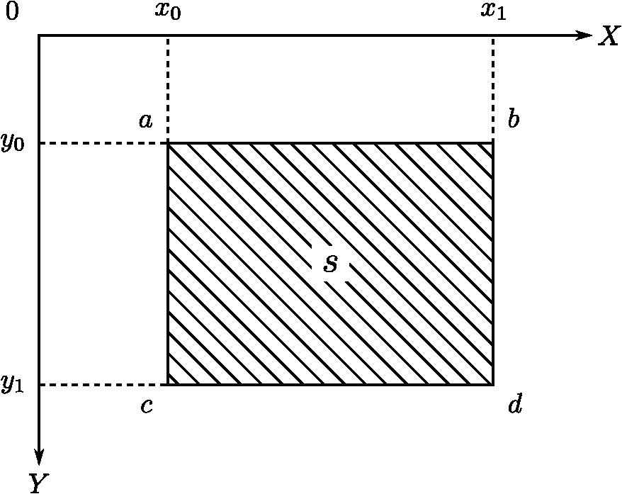
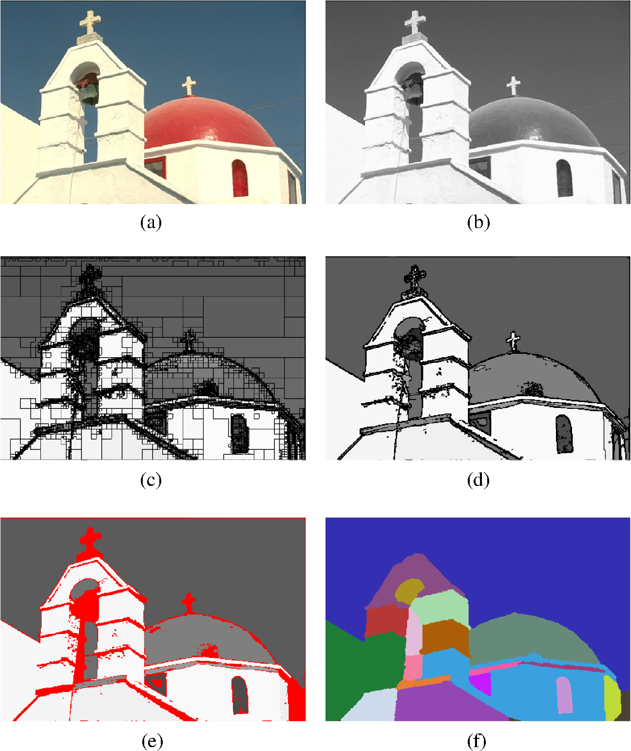
1. Introduction

The segmentation of images is a common procedure in image analysis applications. This procedure is the first step in many processes meant to extract useful information from scenes. It consists of partitioning the image into different disjoint regions that are homogeneous for one or more features computed from the image. Those regions are assumed to correspond to meaningful parts of the objects in the scene, regions that are easier to analyze. In their survey, Vantaram and Saber¹ classify the segmentation methodologies in three main classes: spatially blind, spatially guided, and miscellaneous methods.

As their name suggest, the segmentation of images using the spatially blind methods is not guided by the spatial relationships of the pixels in the image. These methods include approaches using clustering or histogram thresholding. The spatially blind methods have the advantage of being easy to implement and not requiring any a priori information. However, the number of clusters to use for clustering must be determined in advance. This has proven to be a challenging task. Moreover, the histogram thresholding methods have problems with low-contrast images and are difficult to use in color images.

The segmentation of images using spatially guided methods is directed by the relationships between pixels in an image region. These methods group regions that are homogeneous regarding a given image feature. The spatially guided methods are further subdivided into region-based, energy-based, and region and contour-based methods. The region-based methods include procedures such as the growing, the splitting, and the merging of regions. Some algorithms from this category include the J-segmentation algorithm, proposed by Deng and Manjunath,² the gradient segmentation algorithm, proposed by Ugarriza et al.,³ and a multiresolution extension of the gradient segmentation algorithm, proposed by Vantaram et al.,⁴ among others. The energy-based methods attempt to minimize cost functions that model regions in the image. Those cost functions may be contour- or region-based functions. The regions covered by the functions evolve until a given energy model is minimized. Some algorithms in this category include the active contours (a.k.a. snakes), first proposed by Kass et al.⁵ and variants, such as the fast active contours algorithm proposed by Chan and Vese⁶ or the active contours without edges, proposed by Vantaram and Saber.⁷ Finally, the contour-based methods consist of different variants of the watershed algorithm. This algorithm considers a gray-scale image as a topographic relief, where the intensity of the pixels determines the corresponding height of that particular zone. The relief is then flooded in a simulation and the water flows to local minima and forms basins, corresponding to different regions in the image. Some examples of these methods include the work of Gao et al.,⁸ where watersheds are used to segment color images, the study of Hill et al.⁹ that uses a texture gradient to partition textured regions using watershed, and the method by Kim and Kim,¹⁰ where a multiresolution watershed segmentation using wavelets is presented.

In this study, we propose a methodology called integral split and merge (ISM) segmentation. This methodology is a region-based segmentation algorithm, where the split-and-merge segmentation and an image representation called integral image are combined to achieve two main goals: to obtain acceptable segmentation outcomes and to attain a computational complexity low enough to use the method in real-time applications (i.e., 15 fps or more). The split-and-merge segmentation was proposed by Horowitz and Pavlidis¹¹^,¹² in 1974. It consists of recursively partitioning an image into homogeneous parts and then merging those parts into bigger homogeneous regions. Our ISM methodology uses the integral images to improve the computing time performance. The integral image representation was first used in the object recognition field by Viola and Jones,¹³ to achieve a fast feature evaluation for real-time face detection applications.

The proposed ISM method works over intensity images, where the pixels in the homogeneous regions have similar intensity values. The method consists of two main parts: the splitting and the merging steps. The splitting process divides the image into homogeneous regions. This process is performed in a single step, using a quad-tree search. The image is partitioned into regions (i.e., quads) that are evaluated for homogeneity. Because determining the homogeneity of a region is computationally expensive, we use the integral images to improve the time performance. On the other hand, the merging process combines the homogeneous regions obtained from the splitting process, into bigger areas. We propose a merge criterion that is performed in an efficient time and exhibits three main properties. First, it assigns different labels to spatially disconnected regions, independent of their similitude. This is equivalent to performing a connected-component analysis. Second, our method is able to follow gradients in image areas showing this property and group them into single regions. This process is similar to that performed by region-growing methods. Last, our merging procedure is able to automatically determine the number of disjoint regions in the segmentation.

In addition to the ISM split and merge processes, a small-region elimination procedure is presented. This procedure is used to improve the visual appeal of image segmentations, if required. This step first removes the small regions obtained from the ISM segmentation. Then the removed pixels are reassigned to bigger regions using a region growing process. The tests performed show that the small regions have no significant impact in the overall evaluation of a segmentation, therefore, this step may be omitted if necessary.

The ISM methodology was tested to ascertain its performance in segmentation accuracy and computing time. The tests were performed on a collection of natural images where texture patterns are abundant. For this kind of image, it is better to use texture information for the segmentation. Different image features (e.g., texture descriptors) may be used to obtain an intensity map that shows different homogeneity properties. In this work, we use a single texture descriptor: the standard deviation (SD) map. We calculate the SD map in a preprocessing stage. This preprocessing transforms texture features into intensity values that are suitable to be used by our ISM methodology. The SD image describes texture as intensity levels, where each pixel in the SD image is the standard deviation of the intensity values in a neighborhood, centered at the given pixel position in the original image. The ISM methodology used on SD images produces segmentations where the regions are uniform in regard to the standard deviation of their values. Even though there may be better texture descriptors than the SD images, their study is beyond the scope of this work. Here, the SD images are used only to present the ISM methodology. However, despite its simplicity, the SD images have obtained good results in segmentation applications, as in the work of Lizarraga-Morales et al.¹⁴

The results obtained were evaluated using the normalized probabilistic random (NPR) index. The NPR index is a robust methodology developed by Unnikrishnan et al.¹⁵^,¹⁶ to evaluate the quality of image segmentations. The image segmentations obtained from a given algorithm are normally compared against one or more human-made references. To this end, we use the Berkeley segmentation dataset and benchmark (BSDS),¹⁷ a collection of 300 natural images and several human-made segmentation references for each image. The BSDS has been previously used along with the NPR index. An example is the work of Pantofaru and Hebert,¹⁸ where the BSDS and the NPR index are used to evaluate image segmentations, obtained using mean-shift, the efficient graph-based segmentation proposed by Felzenszwalb and Huttenlocher,¹⁹ and a hybrid method that combines both, in order to determine if the hybrid method improves the segmentation quality. The NPR index and the BSDS were also used by Vantaram and Saber¹ to evaluate the segmentation quality of 11 state-of-the-art algorithms. In this study, we compare, in equal terms, the results obtained using our ISM methodology and the results obtained from the 11 algorithms, reported by Vantaram and Saber.¹

The results obtained from the tests performed show that our ISM methodology obtains a similar segmentation quality to the other state-of-the-art algorithms that are used for comparison purposes. However, while the other methods combine both color and texture features, our ISM methodology only requires a single texture feature (i.e., the SD image) to achieve similar results. Furthermore, our tests show that using integral images to calculate the statistics required by the split and merge segmentation improves the execution time of the method. We have found that the ISM methodology is efficiently executed in a piecewise linear time. These contributions may be advantageous for real-time segmentation applications.

The rest of this paper is organized as follows. In Sec. 2, the proposed segmentation methodology is described. Then, performance evaluation and parameter optimization procedures are discussed in Sec. 3. Finally, some concluding remarks are presented in Sec. 4.

2. Methodology

In this section, the proposed split and merge segmentation methodology is described. The section starts by discussing the integral images that are adapted to this particular application. Then the splitting and merging procedures of our methodology are described along with their implementation details. Additionally, two more procedures that may be used after the segmentation are discussed. The first one is a procedure that declassifies small regions, and the second one is a region growing procedure that assigns the declassified pixels to the remaining classes.

2.1.

Integral Images

The proposed ISM methodology makes use of the integral images to improve the time required to obtain an image segmentation. This procedure is essential, because it allows the ISM method to be executed in real time.

The integral images¹³ (a.k.a. summed area tables) are used to efficiently compute sums of pixel intensities in square regions of an image. The time required to compute such sums is constant and does not depend on the region size. Moreover, the integral image may be computed in linear time.

This section describes the method to compute the integral image and to obtain the area sums. These sums are used to compute the mean intensity and the variance of the intensities in an image region. These statistics are used by our splitting process to improve the execution time.

2.1.1.

Summed area table

The integral image, or summed area table, is obtained from the original image and has the same dimensions. This image representation is used to efficiently compute the sum of intensities in a square area of the image.

Let $I$ be an image consisting of $W \times H$ pixels. Also, consider the pixel (0,0) to be at the top-left corner of the image and the pixel ( $W - 1$ , $H - 1$ ) at the bottom-right corner. The pixel at column $i$ and row $j$ in $I$ is denoted by $I (i, j)$ . The integral image $S$ consisting of $W \times H$ cells is calculated, as shown in Eq. (1). The cell at column $i$ and row $j$ in $S$ is denoted by $S (i, j)$ . Each cell $S (i, j)$ is the sum of all the intensities above and to the left of its corresponding image pixel $I (i, j)$ , including itself. The computation of $S (i, j)$ may be optimized using the data already computed, as shown in Eq. (2).

Eq. (1)

S (i, j) = \underset{j^{'} \leq j}{\sum_{i^{'} \leq i}} I (i^{'}, j^{'})

Eq. (2)

S (i, j) = I (i, j) + S (i - 1, j) + S (i, j - 1) - S (i - 1, j - 1)

The function $S (i, j) = 0$ for the values $i$ , $j < 0$ . Notice that using Eq. (2), the integral image is obtained in linear time $O (n)$ .

2.1.2.

Sum of intensities in a region

The integral image may be used to compute the sum of pixel intensities of a square region of arbitrary size. The time required to compute this sum is constant, and it is independent of the size of the area involved.

Consider a square area defined by $a = (x_{0}, y_{0})$ , $b = (x_{1}, y_{0})$ , $c = (x_{0}, y_{1})$ and $d = (x_{1}, y_{1})$ , where $x_{0}$ , $y_{0}$ , $x_{1}$ , and $y_{1}$ are integer numbers representing the coordinates of the region in the image (see Fig. 1). Then, the sum of the pixel intensities ( $s$ ) in the region is obtained using Eq. (3).

Eq. (3)

s = S (x_{1}, y_{1}) - S (x_{0} - 1, y_{1}) - S (x_{1}, y_{0} - 1) + S (x_{0} - 1, y_{0} - 1)

Fig. 1

Area to sum in a summed area table.

The function $S (i, j) = 0$ for the values $i$ , $j < 0$ . Notice that the computation of the Eq. (3) is obtained in constant time $O (1)$ .

2.1.3.

Fast computation of statistics

In their article, Bradley and Roth²⁰ use the integral image to compute the mean intensity of a rectangular region of an image. In this work, a similar approach is used to calculate the mean. Additionally, we also calculate the variance of the pixel intensities in square regions of arbitrary size by using statistical moments.

First, consider Eq. (4), where $s_{r}$ is the sum of all the intensity values, raised to the power of $r$ , in a region defined by $x_{0}$ , $y_{0}$ , $x_{1}$ , and $y_{1}$ . The mean $μ$ and variance $σ^{2}$ of the region data may be computed as a function of $s_{r}$ , using Eqs. (5) and (6), respectively.

Eq. (4)

s_{r} = \sum_{j = y_{0}}^{y_{1}} \sum_{i = x_{0}}^{x_{1}} I^{(r)} (i, j)

Eq. (5)

μ = \frac{s_{1}}{N}

Eq. (6)

σ^{2} = \frac{s_{2}}{N} - {(\frac{s_{1}}{N})}^{2},

where

s_{1} = s_{r = 1}

and

s_{2} = s_{r = 2}

. Notice that the sum

s_{r}

may be efficiently computed using integral images. First, the summed area table of an image with intensities raised to the power of

r

is calculated as shown in Eq. (7).

Eq. (7)

S_{r} (i, j) = I^{(r)} (i, j) + S_{r} (i - 1, j) + S_{r} (i, j - 1) - S_{r} (i - 1, j - 1)

This operation is also performed in linear time $O (n)$ . Then, the sum of intensities $s_{r}$ is calculated using the summed area table $S_{r}$ , as shown in Eq. (8).

Eq. (8)

s_{r} = S_{r} (x_{1}, y_{1}) - S_{r} (x_{0} - 1, y_{1}) - S_{r} (x_{1}, y_{0} - 1) + S_{r} (x_{0} - 1, y_{0} - 1)

The function $S_{r} (i, j) = 0$ for the values $i$ , $j < 0$ . The computation of Eq. (8) is also performed in constant time $O (1)$ .

2.1.4.

Optimization details

The integral images discussed in this section are intended to be used for image segmentation, and because the intensity values of the image pixels are integer (in [0,255]), an integer integral image may be used. This data representation may be advantageous, because the integer arithmetic is faster than the floating point arithmetic. Thus, the segmentation methodology discussed in this work may be fully implemented using only integer arithmetic. Even though the mean and variance values obtained from pixel intensities may be real numbers, an integer approximation is acceptable. Therefore, the division operations required to calculate the mean and the variance may be performed using integer arithmetic alone. Moreover, the division operations required by the splitting process described next may be replaced by bit shifts.

2.2.

Splitting Process

The first step of the proposed segmentation methodology is a splitting process. This process divides the image into regions of homogeneous intensity. First, the image is divided into quads and each quad is tested for homogeneity. If the region is not homogeneous, that region is further subdivided into quads, and the process is repeated until the homogeneity condition is reached, or until a stop condition is met.

A region homogeneous in intensity is a region in the image that has the same intensity for all its pixels. In practice, this situation rarely occurs. Small differences between pixel intensities are expected in perceptually homogeneous regions. Therefore, a certain tolerance to intensity variation may be allowed for homogeneous regions. The maximum intensity variation allowed is determined by a variance threshold ( $σ_{T}^{2}$ ) that is required to be calculated for each image. To that end, an automatic method to detect the variance threshold is also discussed in this section.

2.2.1.

Quad-tree building

Before starting the subdivision process, the original image should be slightly modified in order to make the subdivision easier. First, it results more convenient if the image is square, with sides that are powers of two. This assures the image to be divisible at every level of the tree, and the divided regions to be always powers of two.

If the original image does not meet the aforementioned size requirements, the image canvas is enlarged, adding empty pixels to the right and to the bottom of the image, until obtaining an image of $2^{ℓ} \times 2^{ℓ} pixels$ , where $ℓ$ is a positive integer value such that $2^{ℓ - 1} < \max (W, H) \leq 2^{ℓ}$ . Additionally, it is recommended to assign a special value to the empty pixels. This special value has the property of being always different from any other pixel intensity, regardless of the variance threshold ( $σ_{T}^{2}$ ) used. This way, the empty pixels can only be grouped together, and the space added by the canvas enlargement does not interfere with the segmentation process.

2.2.2.

Subdivision process

The subdivision process starts with the whole image after the canvas enlargement step. Because the side length of the image equals $2^{ℓ}$ , consider the number of levels in quad three to be $ℓ$ .

The homogeneity of the level $ℓ$ of the image is determined by obtaining the variance of the region (in this case the variance of the whole image) and comparing it against the variance threshold $σ_{T}^{2}$ . The variance of the region is efficiently computed by our ISM methodology using integral images, applying Eq. (6). Notice that, for this equation $N = {(2^{ℓ})}^{2} = 2^{2 ℓ}$ , yielding a number that is also a power of two, therefore, the variance calculation requires no division operations, and a bit shift may be used instead.

To decide if the region (in this case the whole image) is homogeneous, its variance should be below the variance threshold level $σ_{T}^{2}$ . Otherwise, the region is considered nonhomogeneous, and is subdivided into four square regions of side $2^{ℓ - 1}$ .

The process is repeated for each one of the four regions. If a region is nonhomogeneous, the region is further subdivided. The process is repeated until the homogeneity condition is met, or the level $ℓ = 0$ is reached. At this point, all the image is divided into different regions that are homogeneous in intensity.

Additionally, the process may be initiated or finalized at arbitrary levels. For example, the splitting process may start at level $ℓ$ . However, until the level $ℓ - α$ is reached, all the regions are considered nonhomogeneous. This consideration is used to avoid segmentation errors produced by big regions containing small areas that should be assigned to a different class. If the mean intensity of such a region is below $σ_{T}^{2}$ , the error may not be detected. However, as mentioned by Ojala and Pietikäinen,²¹ smaller initial regions are easily merged together again by the merging process. In this work, we use a maximum region of $2^{6} \times 2^{6} pixels$ to avoid this kind of error. On the other hand, the process may also be finalized before the level $ℓ = 0$ is reached. This may speed up the subdivision process, because the lower levels in quad three have more regions to process than the upper levels. However, doing this increases the error in the detection of the boundaries between regions, reducing the quality of the segmentation. For this reason, in this work, we use $ℓ = 0$ .

In our implementation, we use a data structure called “node,” to store the information of a given homogeneous region. This information is used to further reduce the operations required by the splitting process. The nodes are stored in a vector as soon as the homogeneous regions are found. Because the quad tree is explored using a breadth-first search, the resulting vector is sorted. This is required by the merging process.

2.2.3.

Automatic variance threshold selection

It is often inconvenient to define a constant variance threshold $σ_{T}^{2}$ for all images, because the optimum variance threshold is dependent on the image under segmentation. In their article, Ugarriza et al.³ propose an automatic approach, called “adaptive gradient thresholds,” that initializes the seeds of their region growing segmentation methodology. We adapted this methodology to determine the best value of $σ_{T}^{2}$ from a gradient map obtained from a given image. This process is fast and should be performed for every image before starting the segmentation. The methodology adapted from the work of Ugarriza et al.³ is discussed in this section.

An estimation of $σ_{T}^{2}$ may be obtained using the next procedure. First, a gradient image is obtained from the original image, which is assumed to have only one channel. The image consists of $K = W \cdot H pixels$ of intensity $U = {u_{1}, u_{2}, u_{3}, \dots, u_{K}}$ , while the gradient image is made of $K = W \cdot H$ values $G = {g_{1}, g_{2}, g_{3}, \dots, g_{K}}$ , for an image of $W \times H pixels$ , where each $k$ index from the $u_{k}$ and $g_{k}$ values corresponds to the image position $k = W j + i$ .

The value for each pixel in the gradient image $G$ is defined as $g = \sqrt{λ}$ , where $λ$ is obtained using Eq. (9) presented by Ugarriza et al.³

Eq. (9)

λ = \frac{1}{2} [q + h + \sqrt{{(q + h)}^{2} - 4 (q h - t^{2})}] .

The variables $q$ , $t$ , and $h$ are defined in Eqs. (10), (11) and (12), respectively. The variables $x$ and $y$ are the spatial coordinates of the image.

Eq. (10)

q = {(\frac{d u}{d x})}^{2}

Eq. (11)

t = (\frac{d u}{d x} \cdot \frac{d u}{d y})

Eq. (12)

h = {(\frac{d u}{d y})}^{2}

The differential terms of Eqs. (10)–(12) are calculated as functions of image intensity values, as shown in Eqs. (13) and (14).

Eq. (13)

\frac{d u}{d x} = I (i, j) - I (i - 1, j)

Eq. (14)

\frac{d u}{d y} = I (i, j) - I (i, j - 1)

After obtaining the gradient image $G$ , its histogram is calculated, and the threshold variance $σ_{T}^{2}$ is obtained from this histogram. It is required to find a threshold $p$ in the histogram where a given percentile is reached. For convenience, the threshold $p$ is normalized in [0,1] and not in [0,100] as is the percentile, but still reflecting the same proportion. The threshold $p$ signals the maximum intensity deviation that should be considered as homogeneous, which is equivalent to $σ_{T}$ (see Fig. 2). Even though $p$ is also a threshold value, its behavior is different from $σ_{T}^{2}$ . While $σ_{T}^{2}$ changes from image to image, $p$ is a constant that may be experimentally determined. Ugarriza et al.³ reported that the optimum value for their adaptive gradient threshold is near 0.8. We experimentally obtained a similar value for the gradient threshold $p = 0.82$ ; the protocol used for this experiment is discussed in Sec. 3.3.1.

Fig. 2

Histogram of the gradient image showing the $p$ threshold level.

2.3.

Merging Process

The ISM merging process combines the homogeneous regions obtained from the splitting process into bigger regions that are assigned to a class. The regions in a class should be homogeneous in intensity and be spatially connected. The ISM merging methodology proposed here has three main characteristics: the number of classes is automatically determined for each image, smooth gradients are considered as homogeneous regions, and different classes are assigned for disconnected regions. The details of our ISM merging algorithm are discussed next.

2.3.1.

Conditions and cases

The homogeneous regions identified by the splitting process (nodes) may be merged together if they fulfill the next merging conditions. First, an unclassified region is always merged into a classified region. Second, the unclassified region should be equal in size or smaller than the region into which it is going to be merged. Third, the difference of the mean intensities between the classified and the unclassified regions should not be greater than $σ_{T}$ . Last, the regions must be adjacent in the vertical and horizontal directions only.

If a region is not classified and has no classified neighbors that fulfill the merging conditions, a new class is created for that region. Additionally, an unclassified region may have more than one adjacent region that fulfills the aforementioned conditions. There may be up to four suitable neighbors for each unclassified region, because of the second merging condition. If those regions share the same class label, the assignment of the region to that class is straightforward. However, if the adjacent regions have different class labels, those labels need to be reassigned to a single class.

2.3.2.

Class assignment

At the beginning of the merging process, there is no class assigned to any region. In this case, and whenever a region has no neighbors that meet any of the merging conditions, a group structure ( $g_{w}$ ) is generated. All the neighboring nodes ( $n_{i}$ ) that fulfill the merging conditions are pointed to a group structure (see Fig. 3). This structure keeps a record of the sum of the pixel intensities from all the nodes.

Fig. 3

Graphic representation of the node ( $n_{i}$ ) and group ( $g_{w}$ ) structures. The arrows depict pointers to structures.

Whenever a new node is created, a new class ( $C_{j}$ ) structure is also defined, and the group is pointed to that class structure. The class contains a unique label and stores a vector containing all the group structures that point to the class. If two or more regions of different classes are merged together, their corresponding groups are added to the group vector of the class. This reduces the computing time otherwise used in node reassignment. Figure 4 shows the relationship between the class and group structures.

Fig. 4

Graphic representation of the group and class structures. The arrows depict pointers to structures.

The merging process is performed using the vector of node structures generated during the splitting process. This vector is sorted by the size of the regions, where the first nodes correspond to the biggest homogeneous regions in the image. This means that all the classes are started using the biggest region possible and smaller regions are added later.

The use of intermediate group structures between the node and the class structure is useful for the implementation only. It considerably reduces the number of operations that are required to merge multiple classes together. At the end of this process, the remaining classes are labeled from 1 to $L$ , consecutively.

2.4.

Small-Region Elimination

At the end of the split and merge segmentation process, all the pixels in the image are assigned to a class in the resulting segmentation. However, there are many classes among them that are associated only with a small group of pixels.

Normally, it is expected that an image segmentation will have a reduced number of classes, and those classes are expected to group the important areas in the image. For this reason, an excess of small classes may pose a problem for some applications. It may be convenient to eliminate those small classes and later reassign their pixels to bigger classes. The elimination process is straightforward. All the class structures are inspected and if the number of pixels associated to that class is below $M$ pixels, the class is eliminated along with the structures used by it. All the pixels affected are declassified.

If elimination of small classes is used, it is more convenient to perform the class labeling afterwards.

2.5.

Region Growing

The declassified pixels from the small region elimination procedure are reassigned to the class that is more convenient with a region growing procedure. Considering that most of the pixels are already classified, the time required to perform this operation should be short, because the region growing is applied only to a small number of pixels.

The process starts by introducing all the unclassified pixels into an FIFO stack. Each element of the queue is tested in order to determine if that particular pixel may be assigned to a neighboring class. There are two conditions to meet in order to perform that assignment. First, the pixel should be a neighbor of a pixel that is already classified. Second, the pixels recently assigned to a class by this process are not considered as classified pixels.

Those pixels that do not meet the assignment conditions are pushed to another FIFO stack to start a second cycle. The pixels that were assigned in the previous step are now considered as classified pixels. This distinction is made in order to make the regions to grow in layers. The same process is repeated until no unclassified pixels remain.

To summarize the ISM segmentation algorithm presented in this section, a series of examples obtained from each step of the methodology are shown in Fig. 5. Figure 5(a) shows the original image. Then, Fig. 5(b) shows the intensity values obtained from the original image, used here as a descriptor. Figure 5(c) shows the homogeneous regions obtained from the splitting process. Their boundaries are shown in black. Figure 5(d) shows the homogeneous regions obtained after the merging process. The boundaries are also shown in black. Figure 5(e) shows in red the small regions containing less than $M$ pixels. Finally, Fig. 5(f) shows the resulting segmentation, obtained after the region growing procedure. This image shows each class label in a different color.

Fig. 5

Segmentation steps: Original image (a), feature description image (b), image after the splitting process (c), image after the merging process (d), elimination of small regions (e), and the resulting segmentation classes obtained after the region growing procedure (f).

3. Tests and Results

This section presents the results obtained from of a series of tests, divided into three categories. The first set of tests is made to determine the optimum segmentation parameters for the proposed algorithm. The second one compares the outcome of the proposed methodology with other state-of-the-art segmentation algorithms. The third set is made to experimentally ascertain the execution time of the method.

It is desirable that the proposed methodology reaches results similar to other state-of-the-art methods. Also, the methodology proposed is expected to be fast enough to be used in real-time applications (i.e., 15 fps or more). Our algorithm is compared with the 11 segmentation methods presented in the survey made by Vantaram and Saber.¹ These algorithms are: the Edge Detection and Image Segmentation (EDISON) system by Christoudias et al.,²² the Compression-based Texture Merging (CTM) by Yang et al.,²³ the J-Segmentation (JSEG) algorithm by Deng and Manjunath,² the Dynamic Color Gradient Thresholding (DCGT) by Balasubramanian et al.,²⁴ the Gradient Segmentation (GSEG) algorithm by Ugarriza et al.,³ a multiresolution extension of the GSEG methodology called MAPGSEG by Vantaram et al.,⁴ the Level Set-based Segmentation (LSS) by Sumengen,²⁵ the Gibbs Random Field (GRF) algorithm by Vantaram and Saber,⁷ the Graph-based Segmentation (GS) algorithm by Felzenszwalb and Huttenlocher,¹⁹ the Ultra-metric Contour Map (UCM) segmentation by Arbeláez and Cohen,²⁶ and a Color Texture Segmentation (CTS) by Hoang et al.²⁷ These segmentation algorithms are evaluated using the normalized probability rand (NPR) index proposed by Unnikrishnan et al.¹⁵ The NPR index requires reference segmentations to determine the evaluation measure, and the Berkeley Segmentation Dataset and Benchmark (BSDS) proposed by Martin et al.¹⁷ is used for that purpose. This is a collection of 300 natural images that includes from 5 to 10 human-made segmentations for each image.

Our ISM algorithm is also evaluated using the NPR index and the BSDS images in order to compare our results with those from the 11 algorithms of the survey under equal conditions. Additionally, to ascertain the significance of the results obtained, a statistical t-test was performed. The test protocols explaining the different experiments are presented next, along with a discussion of the obtained results.

3.1.

Evaluation of Results, Using the NPR Index

The segmentations resulting from the tests performed were evaluated using the NPR index, a segmentation evaluation methodology proposed by Unnikrishnan et al.¹⁵ This methodology compares an image segmentation against a reference segmentation (i.e., the ideal outcome) and determines their similitude. The NPR index has four desirable properties for segmentation evaluation: first, the method is able to compare segmentations that have a different number of regions. This property is important, because the ISM segmentation methodology automatically determines the number of labels of a segmentation and may differ from the references or the results from other algorithms. Second, the NPR index presents no degenerate cases in which bad segmentations obtain abnormally good results. Third, the NPR index is able to use multiple segmentation references to obtain a more objective result and is able to accommodate the refinement of regions found in the references. Finally, the measure obtained from the NPR index allows the comparison between segmentations of different images or between segmentations from different algorithms.

In this work, the Matlab toolkit provided by Yang et al.²³ is used to compute the probabilistic random (PR) index. The required human-made references are provided in the BSDS. The NPR index is obtained using Eq. (15):

Eq. (15)

NPR = \frac{PR - E [PR]}{\max [PR] - E [PR]},

where

\max [PR] = 1

, and

E [PR] = 0.6064

, according to Vantaram and Saber,¹ for the set of 300 natural images in the BSDS.

3.2.

Statistical Tests

For all the tests performed, the segmentation results obtained using the NPR index were averaged. This result is the mean performance of the ISM algorithm over the 300 images in the BSDS. This mean result was compared with the results from the 11 algorithms in the survey of Vantaram and Saber,¹ in order to determine their differences in quality. However, a simple comparison of the mean performance is not enough to provide a conclusion from such comparisons. In cases where the results are too close, the difference may not be significant. In order to identify such cases, statistical significance tests need to be performed for all the comparisons made. In this study, we use a two-sample t-test, where different variances are assumed. Our null hypothesis is that the mean results of two test sets are the same. On the other hand, our alternative hypothesis is that the mean results of two test sets are actually different.

The results obtained are reported in the following sections. Additionally, different tests were performed to optimize the parameter $p$ required by the ISM methodology, the parameter $M$ used for small-region elimination, and the parameter $R$ used in the preprocessing stage to calculate the SD image.

3.3.

Parameter Optimization

This section presents the tests conducted in order to determine the best segmentation parameters for the proposed methodology. There are three parameters to optimize. The first one is the parameter $p$ of the ISM methodology, used to determine the variance threshold $σ_{T}^{2}$ of the image. This parameter specifies the percentile of the image intensities that should be below $σ_{T}^{2}$ in an adaptation of the method proposed by Ugarriza et al.³ The second parameter is the minimum size $M$ allowed for a class in the resulting segmentation. This parameter is used by the small-region elimination process. All pixels of classes below the value of $M$ are declassified and reassigned to bigger classes. The last parameter $R$ defines the size of the window $W = 2 R + 1$ . This window size is required to calculate the SD image of the preprocessing stage. The SD image is used here as a texture descriptor.

3.3.1.

Gradient histogram threshold

The threshold $p$ used to determine the value of $σ_{T}^{2}$ is adapted from the work of Ugarriza et al.³ They report a value of 0.8 for their adaptive gradient thresholds. However, because the adaptation of this method may lead to differences in the results, we conducted a test to independently determine the value of $p$ .

For this test, we used the 300 images from the BSDS proposed by Martin et al.¹⁷ as a training set. All the images in this set were segmented using different values in $0 \leq p \leq 1$ . The segmentation evaluations obtained using the NPR index show that the best value is $p = 0.82$ . Even though this is the best average evaluation value, the statistical significance test performed shows that the differences of the segmentation results are not significant for values in $0.49 < p < 0.88$ , meaning that the method is robust for different values of $p$ . This means that the value of $p = 0.82$ and the value of 0.8 reported by Ugarriza et al.³ for their adaptive gradient thresholds have no significant differences. From now on, we use the value of $p = 0.82$ only as a preference.

3.3.2.

Size of a small region

We conducted a test to determine the optimal value for the minimum class size $M$ used in the small-region elimination step. The 300 testing images from the BSDS were segmented, this time using different values of $M$ that vary from zero to 500 pixels. The results were evaluated using the NPR index and the next results were found.

First, we found that the optimal value obtained is $M = 400$ . However, the statistical significance test performed showed that there is no significant difference in $0 \leq M \leq 500$ . Therefore, the elimination of the small classes is not relevant to ascertain the quality of the image. However, it may be used for display purposes. We choose the value of $M = 400$ for the comparison tests, described in Sec. 3.4.

3.3.3.

Window size to obtain a deviation image

Another test was conducted to determine the optimal size of the inspecting window that was used to obtain the SD image in the preprocessing stage. We used the 300 images in the BSDS to obtain different segmentation sets for different values of $R$ . We average the results from the 300 segmentations for a given $R$ value and then compare the different average results obtained using different $R$ values. The values of $R$ vary in the range of $0 \leq R \leq 20$ . The result obtained shows a maximum for $R = 8$ . However, the statistical significance test shows that the differences are not significant for values in $5 \leq R \leq 12$ . In our implementation, we also used the integral images in the preprocessing stage to calculate the SD image. This has two advantages: first, the SD image is obtained in linear time, and second, that time is independent of the size of the window that is used, i.e., $R$ . Therefore, we can use any value of $R$ without performance losses. We choose $R = 8$ for the performance tests, only as a preference.

3.4.

Segmentation Performance

This section presents the results obtained from the proposed ISM methodology using the SD images as input after the small-region elimination process. Figure 6 shows a diagram of the segmentation process performed using the ISM methodology. The results were compared with other state-of-the-art segmentation methods and were also evaluated using the NPR index.

Fig. 6

Diagram of the segmentation process using the integral split and merge (ISM) methodology.

The evaluation of the segmentations, obtained from the 300 images from the BSDS using the ISM methodology, obtains an average evaluation $μ = 0.390$ , and a standard deviation $σ = 0.636$ . The parameters used were $R = 8$ for the SD image in the preprocessing stage, $p = 0.82$ for the ISM segmentation, and $M = 400$ for the small-region elimination step.

The results from our ISM methodology were compared with the 11 algorithms reported by Vantaram and Saber.¹ Some image examples obtained from these results are shown in Fig. 7. The 11 algorithms used for comparison were applied to the same 300 images from the BSDS as our ISM methodology, and their segmentation results were also evaluated using the NPR index. Therefore, the tests were conducted under the same evaluation conditions.

Fig. 7

Example results: the input image (a), the SD image (b), the segmentation of the SD image using ISM (c), and a human-made reference segmentation (d).

Table 1 shows a comparison of the results obtained by our algorithm and the 11 algorithms. Each algorithm was applied to the 300 images from the BSDS. The resulting segmentations were evaluated using the NPR index. The table shows the mean result for each algorithm ( $μ_{i}$ ), and the standard deviation of the results ( $σ_{i}$ ).

Table 1

Results from the evaluation of the 300 image segmentations, using the NPR index. The table shows the algorithm names (Alg.), a numerical label (i), the mean result (μi), the standard deviation of the sample (σi), and the significance test decision (t-test).

Alg.	$i$	$μ_{i}$	$σ_{i}$	t-test
ISM		0.390	0.636
EDISON	1	0.377	0.383	$μ = μ_{1}$
CTM	2	0.386	0.368	$μ = μ_{2}$
JSEG	3	0.440	0.318	$μ = μ_{3}$
DCGT	4	0.394	0.375	$μ = μ_{4}$
GSEG	5	0.496	0.306	$μ \neq μ_{5}$
MAPGSEG	6	0.495	0.312	$μ = μ_{6}$
LSS	7	0.329	0.344	$μ = μ_{7}$
GRF	8	0.488	0.309	$μ = μ_{8}$
GS	9	0.457	0.324	$μ = μ_{9}$
UCM	10	0.507	0.322	$μ \neq μ_{10}$
CTS	11	0.214	0.419	$μ \neq μ_{11}$

Additionally, the table shows the conclusions obtained from the statistical significance t-test. The mean result of each algorithm used for comparison ( $μ_{i}$ ) was tested against the mean result from our ISM methodology ( $μ$ ). The t-test determines whether the difference between mean values is significant or not. The table shows $μ = μ_{i}$ when the differences are not statistically significant, and $μ \neq μ_{i}$ otherwise.

The results from the t-test show that there are no significant differences between the results obtained from our methodology and the algorithms used for comparison, with the exception of the GSEG and the UCM algorithms that obtain better results and the CTS algorithm that obtains worse results. Therefore, our ISM methodology using the SD image as a texture descriptor obtains results comparable to most of the eleven algorithms tested. However, the use of a feature descriptor other than the SD image may lead to better results.

3.5.

Execution Time and Algorithmic Complexity

An execution time test was performed to determine the complexity of the ISM methodology relevant to the number of pixels processed. For the test, 150 scaled sets of the BSDS were used. The ISM segmentation was applied to all 300 images in each scaled set. The segmentation of each scaled set was repeated 100 times in order to increase the accuracy of the registered time $t$ . This process was repeated for all the 150 scaled versions. Figure 8 shows as dots the time (ms) obtained experimentally for different number of pixels ( $n$ ), corresponding to different scaled versions of the BSDS. The average segmentation time for a typical $n$ -pixel image from the database is obtained by computing $t / 30,000$ .

Fig. 8

Time complexity of the ISM methodology.

The results show a piecewise linear behavior. The discontinuities between segments are related to the canvas enlargement step of the ISM methodology. For nonsquare $W \times H$ image sizes, having $\min (W, H) < 2^{ℓ} / 2$ , two quads are filled only by empty pixels. The processing required for those quads is negligible. However, for images having $\min (W, H) \geq 2^{ℓ} / 2$ , there are no empty quads, and the number of quad divisions increases significantly. The time “jump” occurs for image sizes having $\min (W, H) = 2^{ℓ} / 2 + 1$ . Even though these jumps seem to increase the time consumption, their occurrence decrease in frequency as $n$ increases because the occurrence of the jumps are functions of powers of two.

The results of the different experiments shown as dots in Fig. 8 were adjusted to lines, using the least squares fitting methodology. The tests performed on the 300 images from the BSDS for images of $481 \times 321 pixels$ show that a single image is segmented in an average time of 32.6 ms, using a microprocessor fourth generation Intel Core i7 at 3.40 GHz. Because of its piecewise linear time complexity, the ISM methodology may achieve real-time segmentation using adequate hardware.

4. Concluding Remarks

In this study, we propose the ISM segmentation methodology, a split-and-merge segmentation algorithm that uses integral images to achieve real-time segmentation through the fast computation of statistics. Additionally, the ISM methodology performs connected component analysis. Therefore, regions showing equal features are labeled as different regions if they are not spatially connected. Also, the method is able to follow the gradients present in some image areas and group those areas into a single region. Last, the ISM methodology automatically determines the number of regions in each image segmentation. The comparison of results between our ISM methodology and other state-of-the-art algorithms shows that our ISM methodology obtains results as good as most of the methods evaluated. Even though the results from the GSEG and the UCM algorithms obtained a better performance, the outcomes from the ISM method using a simple SD image as a texture descriptor are comparable to those of the rest of the algorithms. However, this quality is achieved by the ISM method using a single texture feature, while the other methods use a combination of both color and texture features. Additionally, better results may be achieved using different feature descriptors, or by the combination of two or more descriptors. Regarding the execution time, the execution tests show that the ISM methodology is executed with a piecewise linear algorithmic complexity. To our knowledge, none of the comparison algorithms achieves this execution time. Our methodology is able to obtain image segmentations at a rate of about 32 fps for images of $481 \times 321 pixels$ ; in this instance, the application may be considered real-time. The results show that the ISM methodology may be a good alternative for applications that need a fast segmentation using few image features, while still achieving an acceptable segmentation quality.

Acknowledgments

Fernando E. Correa-Tome thanks the Mexican National Council on Science and Technology, CONACyT, for the financial support provided via the scholarship 295697/226942.

This work has been partially funded by the University of Guanajuato via the DAIP project “Características Visuales Relevantes para el Reconocimiento de Objetos,” and the PIFI-2013.

References

1.

S. VantaramE. Saber, “Survey of contemporary trends in color image segmentation,” J. Electron. Imaging, 21 (4), 040901 (2012). http://dx.doi.org/10.1117/1.JEI.21.4.040901 JEIME5 1017-9909 Google Scholar

2.

Y. DengB. Manjunath, “Unsupervised segmentation of color-texture regions in images and video,” IEEE Trans. Pattern Anal. Mach. Intell., 23 (8), 800 –810 (2001). http://dx.doi.org/10.1109/34.946985 ITPIDJ 0162-8828 Google Scholar

3.

L. G. Ugarrizaet al., “Automatic image segmentation by dynamic region growth and multiresolution merging,” IEEE Trans. Image Process., 18 (10), 2275 –2288 (2009). http://dx.doi.org/10.1109/TIP.2009.2025555 IIPRE4 1057-7149 Google Scholar

4.

S. Vantaramet al., “Multiresolution adaptive and progressive gradient-based color image segmentation,” J. Electron. Imaging, 19 (1), 013001 (2010). http://dx.doi.org/10.1117/1.3277150 JEIME5 1017-9909 Google Scholar

5.

M. KassA. WitkinD. Terzopoulos, “Snakes: active contour models,” Int. J. Comput. Vision, 1 (4), 321 –331 (1988). http://dx.doi.org/10.1007/BF00133570 IJCVEQ 0920-5691 Google Scholar

6.

T. ChanL. Vese, “Active contours without edges,” IEEE Trans. Image Process, 10 (2), 266 –277 (2001). http://dx.doi.org/10.1109/83.902291 IIPRE4 1057-7149 Google Scholar

7.

S. VantaramE. Saber, “An adaptive Bayesian clustering and multivariate region merging-based technique for efficient segmentation of color images,” in IEEE Int. Conf. Acoustics, Speech and Signal Processing (ICASSP), 1077 –1080 (2011). Google Scholar

8.

H. GaoW. SiuC. Hou, “Improved techniques for automatic image segmentation,” IEEE Trans. Circuits Sys. Video Tech., 11 (12), 1273 –1280 (2001). http://dx.doi.org/10.1109/76.974681 ITCTEM 1051-8215 Google Scholar

9.

P. HillC. CanagarajahD. Bull, “Image segmentation using a texture gradient based watershed transform,” IEEE Trans. Image Process, 12 (12), 1618 –1633 (2003). http://dx.doi.org/10.1109/TIP.2003.819311 IIPRE4 1057-7149 Google Scholar

10.

J. KimH. Kim, “Multiresolution-based watersheds for efficient image segmentation,” Pattern Recogn. Lett., 24 (1–3), 473 –488 (2003). http://dx.doi.org/10.1016/S0167-8655(02)00270-2 PRLEDG 0167-8655 Google Scholar

11.

S. HorowitzT. Pavlidis, “Picture segmentation by a tree traversal algorithm,” J. ACM, 23 (2), 368 –388 (1976). http://dx.doi.org/10.1145/321941.321956 JOACF6 0004-5411 Google Scholar

12.

S. HorowitzT. Pavlidis, “Picture segmentation by a directed split-and-merge procedure,” in Proc. 2nd Int. Joint Conf. on Pattern Recognition IJCPR, 424 –433 (1974). Google Scholar

13.

P. ViolaM. Jones, “Rapid object detection using a boosted cascade of simple features,” in Proc. IEEE Conf. Computer Vision and Pattern Recognition, 511 –518 (2001). Google Scholar

14.

R. Lizarraga-Moraleset al., “Integration of color and texture cues in a rough set-based segmentation method,” J. Electron. Imaging, 23 (2), 023003 (2014). http://dx.doi.org/10.1117/1.JEI.23.2.023003 JEIME5 1017-9909 Google Scholar

15.

R. UnnikrishnanC. PantofaruM. Hebert, “Toward objective evaluation of image segmentation algorithms,” IEEE Trans. Pattern Anal. Mach. Intell., 29 (6), 929 –944 (2007). http://dx.doi.org/10.1109/TPAMI.2007.1046 ITPIDJ 0162-8828 Google Scholar

16.

R. UnnikrishnanC. PantofaruM. Hebert, “A measure for objective evaluation of image segmentation algorithms,” in Proc. CVPR Workshop Empirical Evaluation Methods in Computer Vision, (2005). Google Scholar

17.

D. Martinet al., “A database of human segmented natural images and its application to evaluating segmentation algorithms and measuring ecological statistics,” in Proc. 8th Int. Conf. Computer Vision, 416 –423 (2001). Google Scholar

18.

C. PantofaruM. Hebert, “A Comparison of Image Segmentation Algorithms,” (2005). Google Scholar

19.

P. FelzenszwalbD. Huttenlocher, “Efficient graph-based image segmentation,” Int. J. Comput. Vision, 59 (2), 167 –181 (2004). http://dx.doi.org/10.1023/B:VISI.0000022288.19776.77 IJCVEQ 0920-5691 Google Scholar

20.

D. BradleyG. Roth, “Adaptive thresholding using the integral image,” J. Graph. GPU Game Tools, 12 (2), 13 –21 (2007). http://dx.doi.org/10.1080/2151237X.2007.10129236 Google Scholar

21.

T. OjalaM. Pietikäinen, “Unsupervised texture segmentation using feature distributions,” Pattern Recognit., 32 (3), 477 –486 (1999). http://dx.doi.org/10.1016/S0031-3203(98)00038-7 PTNRA8 0031-3203 Google Scholar

22.

C. ChristoudiasB. GeorgescuP. Meer, “Synergism in low-level vision,” in 16th IEEE Int. Conf. Pattern Recogn., 150 –155 (2002). Google Scholar

23.

A. Yanget al., “Unsupervised segmentation of natural images via lossy data compression,” Comput. Vision Image Underst., 110 (2), 212 –225 (2008). http://dx.doi.org/10.1016/j.cviu.2007.07.005 CVIUF4 1077-3142 Google Scholar

24.

G. Balasubramanianet al., “Unsupervised color image segmentation using a dynamic color gradient thresholding algorithm,” Proc. SPIE, 6806 68061H (2008). http://dx.doi.org/10.1117/12.766184 PSISDG 0277-786X Google Scholar

25.

B. Sumengen, “A Matlab toolbox implementing level set methods,” (2005) http://barissumengen.com/level_set_methods/ Google Scholar

26.

P. ArbeláezL. Cohen, “A metric approach to vector-valued image segmentation,” Int. J. Comput. Vision, 69 (1), 119 –126 (2006). http://dx.doi.org/10.1007/s11263-006-6857-5 IJCVEQ 0920-5691 Google Scholar

27.

M. HoangJ. GeusebroekA. Smeulders, “Color texture measurement and segmentation,” Signal Process., 85 (2), 265 –275 (2005). http://dx.doi.org/10.1016/j.sigpro.2004.10.009 SPRODR 0165-1684 Google Scholar

Biography

Fernando E. Correa-Tome received his ME degree in electrical engineering in 2011 from the Universidad de Guanajuato, Mexico. He received a BE degree in communications and electronics in 2009, also from the Universidad de Guanajuato. He is currently pursuing his doctoral degree in electrical engineering. His current research interests include image and signal processing, pattern recognition, computer vision, and machine learning.

Raul E. Sanchez-Yanez received a Doctor of Science (optics), from the Centro de Investigaciones en Óptica (CIO), Leon, Mexico, in 2002. He received a master’s in electrical engineering and a BE in electronics, both from the Universidad de Guanajuato, where he has been a full-time professor since 2003 in the Engineering Division of the Irapuato-Salamanca campus. His research interests include color and texture analysis for computer vision and computational intelligence applications in feature extraction and decision making.

CC BY: © The Authors. Published by SPIE under a Creative Commons Attribution 4.0 Unported License. Distribution or reproduction of this work in whole or in part requires full attribution of the original publication, including its DOI.

Citation Download Citation

Fernando E. Correa-Tome and Raul E. Sanchez-Yanez "Integral split-and-merge methodology for real-time image segmentation," Journal of Electronic Imaging 24(1), 013007 (7 January 2015). https://doi.org/10.1117/1.JEI.24.1.013007

Published: 7 January 2015

Access the abstract

JOURNAL ARTICLE
11 PAGES

DOWNLOAD PAPER SAVE TO MY LIBRARY

GET CITATION

CITATIONS

Cited by 5 scholarly publications.

Explore citations on Lens.org

KEYWORDS

Image segmentation

Image processing

Image processing algorithms and systems

Image quality

Detection and tracking algorithms

Visualization

Statistical analysis

1.

Introduction

2.

Methodology