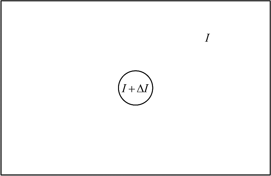
2.1.

Parametric Models

Gaussian mixture model (GMM) and its improved methods: GMM is a classical and probably the most widely used BS technique.¹⁶ GMM models the temporal distribution of each pixel using a mixture of Gaussians, and many studies have proven that GMM can handle gradual illumination changes and repetitive background motion well. In Ref. 17, Lee proposed an adaptive learning rate for each Gaussian model to improve the convergence rate without affecting the stability. In Ref. 18, Zivkovic and Van Der Heijden proposed a scheme to dynamically determine the appropriate number of Gaussian models for each pixel based on observed scene dynamics to reduce processing time. In Ref. 19, Zhang et al. used a spatio-temporal Gaussian mixture model incorporating spatial information to handle complex motions of the background.

Models using other statistical distributions: recently, a mixture of symmetric alpha-stable distributions²⁰ and a mixture of asymmetric Gaussian distributions²¹ have been employed to enhance the robustness and flexibility of mixture modeling in real scenarios, respectively. They can handle the dynamic backgrounds well. In Ref. 22, Haines and Xiang proposed a Dirichlet process Gaussian mixture model which constantly adapts its parameters to the scene in a block-based method.

2.2.

Nonparametric Models

Kernel density estimation (KDE) and its improved methods: a nonparametric technique²³ was developed to estimate background probabilities at each pixel from many recent samples over time using KDE. In Ref. 24, Sheikh modeled the background using KDE over a joint domain-range representation of image pixels to sustain high levels of detection accuracy in the presence of dynamic backgrounds.

Codebook and its improved methods: the essential idea behind the codebook²⁵ approach is to capture long-term background motion with limited memory by using a codebook for each pixel. In Ref. 4, a multilayer codebook-based background subtraction (MCBS) model was proposed. Combining the multilayer block-based strategy and the adaptive feature extraction from blocks of various sizes, MCBS can remove most of the dynamic backgrounds and significantly increase the processing efficiency.

2.3.

Advanced Models

Self-organizing background subtraction (SOBS) and its improved methods: in the 2012 IEEE change detection workshop²⁶ (CDW-2012), SOBS²⁷ and its improved method SC-SOBS²⁸ obtained excellent results. In Ref. 27, SOBS adopted a self-organizing neural network to build a background model, initialized its model from the first frame, and employed regional diffusion of background information in the update step. In 2012, Maddalena improved the SOBS by introducing spatial coherence into the background update procedure, which led to the SC-SOBS algorithm providing further robustness against false detections. In Ref. 29, three-dimensional self-organizing background subtraction (3D_SOBS) used spatio-temporal information to detect a stopped object. Recently, the 3DSOBS+¹ algorithm further enhanced the 3D_SOBS approach to accurately handle scenes containing dynamic backgrounds, gradual illumination changes, and shadows cast by moving objects.

ViBe and its improved methods: in the CDW-2012, ViBe⁸ and its improved method ViBe+³⁰ also achieved remarkable results. Barnich and Van Droogenbroeck proposed a sample-based algorithm that builds the background model by aggregating previously observed values for each pixel location. The key innovation of ViBe is introducing the random policy into the BS, which makes it the first nondeterministic BS method. In Ref. 30, Van Droogenbroeck and Barnich improved ViBe in many aspects, including an adaptive threshold. They computed the standard deviation of background samples of a pixel to define a matching threshold. The matching threshold adapts itself to statistical characteristics of background samples; however, all background samples of a pixel have the same thresholds, and one wrongly updated background sample will affect the thresholds of other background samples, which will lead to more misclassification. In Refs. 30 and 31, a new update mechanism separating “segmentation map” and “updating mask” was proposed. The “spatial diffusion” update mechanism can be inhibited in the “updating mask” to detect still foreground objects. In Ref. 32, Mould and Havlicek proposed an update mechanism in which foreground pixels can update their background models by replacing the most significant outlying samples. This update policy can improve the ability to deal with ghosts.

2.4.

Human Visual System-Based Models

Visual saliency, another important concept about the HVS, has already been used in the BS methods. In Ref. 33, Liu et al. represented object saliency for moving object detection by an information saliency map calculated from spatio-temporal volumes. In Ref. 34, Mahadevan and Vasconcelos proposed a BS algorithm based on spatio-temporal saliency using a center-surround framework, which is inspired by biological mechanisms of motion-based perceptual grouping. These methods have shown the potential of the HVS in moving object detection.

In this paper, we propose an improved BS technique which uses the characteristic of the HVS.

We introduce an adaptive distance threshold into ViBe to simulate the capacity of the HVS in perceiving noticeable intensity changes, which can discriminate camouflaged foreground objects and reduce false negatives. Together with ViBe’s update policy, our method further improves the ability to detect foreground objects that are motionless for a while. Hence, IViBe improves the ability of ViBe in dealing with camouflaged and still foreground objects.

3.1.

Adaptive Distance Threshold

In order to better segment foreground objects similar to the background, we introduce an adaptive distance threshold $R_k(x_i)$ for background matching. Different from ViBe which uses a fixed distance threshold $R_k(x_i)=20$ for each background sample, we propose an adaptive distance metric through simulating the characteristics of human visual perception (i.e., Weber’s law³⁵).

Weber’s law describes the human response to a physical stimulus in a quantitative fashion. The just noticeable difference (JND) is the minimum amount by which stimulus intensity must be changed in order to produce a noticeable variation in the sensory experience. Ernst Weber, a 19th century experimental psychologist, observed that the size of the JND is linearly proportional to the initial stimulus intensity. This relationship, known as Weber’s law, can be expressed as

In visual perception, Weber’s law actually describes the ability of the HVS for brightness discrimination, and the Weber ratio can be obtained by a classic experiment³⁶ which consists of having a subject look at a flat, uniformly illuminated area (with intensity $I$) large enough to occupy the entire field of view, as Fig. 1 shows. An increment of illumination (i.e., $\mathrm{\Delta }I$) is added to the field and appears as a circle in the center. When $\mathrm{\Delta }I$ achieves $\mathrm{\Delta }{I}_{\mathrm{JND}}$, the subject will give a positive response, indicating a perceivable change. In Weber’s law, $\mathrm{\Delta }{I}_{\mathrm{JND}}$ is in direct proportion to $I$. Hence, the $\mathrm{\Delta }{I}_{\mathrm{JND}}$ is small in dark backgrounds and big in bright backgrounds.

Fig. 1

Basic experimental setup used to characterize brightness discrimination.

In the BS methods, when comparing current intensity with the corresponding background model, the distance threshold can actually be considered as the critical intensity difference in distinguishing foreground objects from the background. Fortunately, Weber’s law describes the capacity of the HVS in perceiving noticeable intensity changes, and the JND that the HVS can perceive is in direct proportion to the background illumination. Inspired by Weber’s law, we propose our adaptive distance threshold in direct proportion to the background sample intensity; namely, the distance threshold should be low for a dark background sample and high for a bright background sample.

In our method, mapping to Weber’s law is as follows: the background sample intensity $B_k(x_i)$ can be regarded as the initial intensity $I$, the difference between the current value and each background sample is the intensity change $\mathrm{\Delta }I$, and the distance threshold $R_k(x_i)$ can be regarded as the JND (i.e., $\mathrm{\Delta }{I}_{\mathrm{JND}}$). Consequently, on the basis of Weber’s law, we set

In Eq. (4), $B_k(x_i)$ is the known background sample intensity, and if we want to derive the distance threshold $R_k(x_i)$, we have to first obtain the Weber ratio $c$. However, we cannot directly use the Weber ratio obtained in the classic experiment, because the classic experiment uses a uniformly illuminated area as background, but what we need in our method is a Weber ratio with a complex image as the background. As described in Ref. 37, “for any point or small area in a complex image, the Weber ratio is generally much larger than that obtained in an experimental environment because of the lack of sharply defined boundaries and intensity variations in the background.” Moreover, it is also difficult to gain the Weber ratio via redoing the classic experiment using a complex image as the background, because such an experiment will need many subjects and the subjects’ evaluation criteria are inconsistent, which will reduce the creditability of the experiment.

Based on the consideration above, we employ a substitute of subjective evaluations in the classic experiment to derive the Weber ratio $c$ for a complex image as the background. Specifically, the substitute is the difference of the peak signal-to-noise ratio (PSNR³⁸) presented by the motion picture experts group (MPEG). The MPEG recommends that,³⁸ for an original reference image ($R$) and two of its reconstructed images ($D_1$ and $D_2$), only when the difference of PSNR (i.e., $\mathrm{\Delta }\mathrm{PSNR}$) satisfies

Since $\mathrm{\Delta }\mathrm{PSNR}$ can objectively reflect the ability of the HVS in discriminating intensity changes, we use $\mathrm{\Delta }\mathrm{PSNR}$ to substitute the subjects’ perception in the classic experiment with a complex image as the background. Here, we first construct a complex image. Suppose there is a complex image whose rows and columns are divided into 16 equal parts, respectively. Thus, the complex image is composed of 256 regions of the same size. For each region, the setup is the same as the classic experiment shown in Fig. 1. That is, each region is uniformly illuminated with intensity $I$, and an increment of illumination (i.e., $\mathrm{\Delta }I$) is added to the centered circle. Such a region is called a basic region. The complex image consists of 256 basic regions (with $I=\mathrm{0,1},\dots ,255$), which are randomly permutated, as shown in Fig. 2. In this way, we construct a complex image as the background to simulate the classic experiment in all intensity levels simultaneously, which makes our derivation general and objective.

Fig. 2

Simulated complex image as background.

All the circles in the basic regions of Fig. 2 simultaneously change their intensities with $\mathrm{\Delta }I$. When $|\mathrm{\Delta }I|$ reaches $\mathrm{\Delta }{I}_{\mathrm{JND}}$ for all the basic regions, the HVS can barely perceive the intensity changes of the complex image (let this image be $D_1$). When $|\mathrm{\Delta }I|=\mathrm{\Delta }{I}_{\mathrm{JND}}+\epsilon$ ($\epsilon$ is a very small constant, and for a digital image we set $\epsilon =1$) for all the basic regions, the HVS can obviously perceive the intensity changes of the complex image (let this image be $D_2$). Suppose the complex image shown in Fig. 2 is the original reference image (i.e., $R$), then $D_1$ and $D_2$ can be regarded as two different distorted images which are reconstructed from the same $R$ and are just perceivably distinguishable by the HVS. Accordingly, on the basis of Eq. (3), the 1-norm of difference between $R$ and $D_1$ is given in Eq. (7), and the 1-norm of difference between $R$ and $D_2$ is provided in Eq. (8),

Simplifying Eq. (9), we can derive $c=0.13$. As a result, we conclude that the relationship between the intensity of a background sample and its corresponding distance threshold is: $R_k(x_i)=0.13B_k(x_i)$.

Nevertheless, according to the description of brightness adaptation of the HVS in Ref. 37, we can infer that, in the extremely dark and extremely bright regions of a complex image, the linear relationship in Weber’s law cannot precisely describe the relation between perceptible intensity changes of the HVS and the background illumination. Therefore, our solution is to cut off the distance threshold for background samples whose intensities are too high or too low. After many experiments, we empirically set [10%, 90%] of the entire intensity range satisfying the linear relationship. Namely, the cut off intensities are $T_1=\lceil 255\times 0.1\rceil =26$ and $T_2=\lceil 255\times 0.9\rceil =230$. Consequently, the adaptive distance threshold can be calculated as

Fig. 3

The relationship between the intensity of a background sample and its corresponding distance threshold.

3.2.

Background Model Update Mechanism and Impacts of Our Adaptive Distance Threshold Together with Update Mechanism on Detection Results

It is essential to update the background model $\mathit{B}(x_i)$ to adapt to changes in the background, such as lighting changes and variations of the background. The update of background models is not only for pixels classified as background, but also for their randomly selected eight-connected neighborhood. In detail, when a pixel $x_i$ is classified as background, its current intensity $I(x_i)$ is used to randomly replace one of its background samples $B_k(x_i)$ ($k\in \{\mathrm{1,2},\dots .,N\}$) with a probability $p=1/\varphi$, where $\varphi$ is a time subsampling factor similar to the learning rate in GMM (the smaller the $\varphi$ we use, the faster the update speed we get). After updating the background model of pixel $x_i$, we randomly select a pixel $x_j$ in the eight-connected spatial neighborhood of pixel $x_i$, i.e., $x_j\in N_8(x_i)$. In light of the spatial consistency of neighboring background pixels, we also use the current intensity $I(x_i)$ of pixel $x_i$ to randomly replace one of pixel $x_j$’s background samples $B_k(x_j)$ ($k\in \{\mathrm{1,2},\dots .,N\}$). In this way, we allow a spatial diffusion of background samples in the process of background model update.

The advantage of this “spatial diffusion” update mechanism is the quick absorption of certain types of ghosts (a set of connected points, detected as in motion but not corresponding to any real moving object⁸). Some ghosts result from removing some parts of the background; therefore, those ghost areas often share similar intensities with their surrounding background. When background samples from surrounding areas try to diffuse inside the ghosts, these samples are likely to match with current intensities at the diffused locations. Thus, the diffused pixels in the ghosts are gradually classified as background. In this way, the ghosts can be progressively eroded until they entirely disappear.

However, the “spatial diffusion” update mechanism is disadvantageous for detecting still foreground objects. In environments where the foreground objects are static for several frames, either because the foreground objects share similar intensities with the background, or due to the noise inevitably emerging in the video sequence, some pixels of the foreground objects may be misclassified as background, and then serve as erroneous background seeds propagating foreground intensities in the background models of their neighboring pixels. Since foreground objects are still for several frames, the background models of the neighboring pixels of these misclassified pixels will suffer from more and more incorrect background samples coming from misclassified foreground intensities. In this way, there will be more misclassified foreground pixels, which will lead to the diffusion of misclassification.

Fortunately, our IViBe employs background matching based on an adaptive distance threshold which can reduce the misclassification inside the foreground objects, can slow down the speed of the misclassification diffusion, and can lower the eaten up speed of still foreground objects. First, IViBe makes full use of the adaptive distance threshold to enhance the discriminating power of similar foregrounds and backgrounds, and then reduces the number of misclassified foreground pixels, which can decrease the possibility of erroneous background seeds occurring. Second, even though misclassification emerges inside the foreground objects for some reason and leads foreground intensities diffusing into the background models of neighboring pixels, the adaptive distance threshold can also cut down the misclassification possibilities of those neighboring pixels inside the foreground objects. Via the aforementioned analysis, we conclude that IViBe has the ability to detect still foreground objects that are present for several frames.

Since we use the adaptive distance threshold as Eq. (10), our threshold for dark areas will be smaller than that of ViBe, hence fewer pixels will be classified as background and then be updated; whereas for bright areas, our threshold will be larger than the fixed threshold used by ViBe, and so more pixels will be classified as background and will then be updated. Accordingly, the updating probability is lower for dark areas and higher for bright areas.

4.1.

Experimental Setup

4.1.2.

Determination of parameter setting

There are six parameters in IViBe: number of background samples stored in each pixel’s background model (i.e., $N$), ratio of $R_k(x_i)$ to $B_k(x_i)$ (i.e., $c$), cutoff thresholds (i.e., $T_1$ and $T_2$), required number of close background samples when classifying a pixel as background (i.e., ${\#}_{\min }$), and time subsampling factor (i.e., $\varphi$).

In Sec. 3.1, we have determined the parameters of our adaptive distance threshold, namely $c=0.13$, $T_1=26$, and $T_2=230$.

In order to evaluate ${\#}_{\min }$ and $N$ with a variety of values, we introduce the metric called percentage of correct classification⁸ (PCC) that is widely used in computer vision to assess the performance of a binary classifier. Let TP be the number of true positives, TN be the number of true negatives, FP be the number of false positives, and FN be the number of false negatives. These raw data (i.e., TP, TN, FP and FN) are summed up over all the frames with ground-truth references in a video. The definition of PCC is given as follows:

Eq. (11)

$$\mathrm{PCC}=\frac{100(\mathrm{TP}+\mathrm{TN})}{\mathrm{TP}+\mathrm{FP}+\mathrm{TN}+\mathrm{FN}}.$$

Figure 4 illustrates the evolution of the PCC of IViBe on the pedestrians sequence (with 800 ground-truth references) in the baseline category for ${\#}_{\min }$ ranging from 1 to 20. The other parameters are fixed to $N=20$, $c=0.13$, $T_1=26$, $T_2=230$, and $\varphi =16$. As shown in Fig. 4, when the ${\#}_{\min }$ increases, the PCC goes down. The best PCCs are obtained for ${\#}_{\min }=1$ ($\mathrm{PCC}=99.8310$), ${\#}_{\min }=2$ ($\mathrm{PCC}=99.8324$) and ${\#}_{\min }=3$ ($\mathrm{PCC}=99.7923$). In our experiments, we find that for stable backgrounds like those in the baseline category, ${\#}_{\min }=1$ can also lead to excellent results. But in more challenging scenarios, ${\#}_{\min }=2$ and ${\#}_{\min }=3$ are good choices. Since a rise in ${\#}_{\min }$ is likely to increase the computational cost of IViBe, we set ${\#}_{\min }=2$.

Fig. 4

PCCs for ${\#}_{\min }$ ranging from 1 to 20.

Once we set ${\#}_{\min }=2$, we study the influence of the parameter $N$ on the performance of IViBe. Figure 5 shows the percentages obtained on the pedestrians sequence for $N$ ranging from 2 to 30. The other parameters are fixed to ${\#}_{\min }=2$, $c=0.13$, $T_1=26$, $T_2=230$, and $\varphi =16$. We observe that higher values of $N$ provide a better performance. However, the PCCs tend to saturate for $N\ge 20$. Considering that a large $N$ value will induce a large memory cost, we select $N=20$.

Fig. 5

PCCs for $N$ ranging from 2 to 30.

The time subsampling factor $\varphi$ is just like the learning rate in the GMM. A large time subsampling factor indicates a small update probability, then the background samples are unable to timely adapt to changes in the real backgrounds, such as gradual illumination changes. That is, when using a large $\varphi$, there may be more false positives due to the outdated background model. On the contrary, a small $\varphi$ means that the background samples are very likely to be updated according to the current frame, and a still foreground object may be much easier to be absorbed into the background to produce more false negatives. Hence, there is a trade-off to adjust $\varphi$ in order to balance the false positives and the false negatives. Besides, $\varphi$ also affects the speed of our method, because a small $\varphi$ will lead to a much higher computational cost for updating. As in ViBe, we also set $\varphi =16$.

Therefore, the parameters of IViBe are set as follows: the number of background samples stored in each pixel’s background model is fixed to $N=20$; the ratio of $R_k(x_i)$ to $B_k(x_i)$ is set to $c=0.13$; the cutoff thresholds are set to $T_1=26$ and $T_2=230$; the required number of close background samples when classifying a pixel as background is fixed to ${\#}_{\min }=2$; the time subsampling factor is fixed to $\varphi =16$.

As for ViBe, the recommended parameters as suggested in Ref. 8 have been used: $N=20$, $R_k(x_i)=20$, ${\#}_{\min }=2$, and $\varphi =16$.

4.2.

Visual Comparisons

For qualitative evaluation, we visually compare the detection results of our IViBe with those of ViBe in Figs. 6Fig. 7Fig. 8Fig. 9–10 on the test sequences. Although multiple test frames were used for each test sequence, we only show one typical frame for each sequence here due to space limitation.

Fig. 6

Detection results of the lakeSide sequence: (a) frame 2255 of the lakeSide sequence, (b) ground-truth reference, (c) result of ViBe, (d) result of IViBe.

Fig. 7

Detection results of the blizzard sequence: (a) frame 1266 of the blizzard sequence, (b) ground-truth reference, (c) result of ViBe, (d) result of IViBe, (e)–(h) partial enlarged views of (a)–(d).

Fig. 8

Detection results of the library sequence: (a) frame 2768 of the library sequence, (b) ground-truth reference, (c) result of ViBe, (d) result of IViBe.

Fig. 9

Detection results of the sofa sequence: (a) frame 900 of the sofa sequence, (b) ground-truth reference, (c) result of ViBe, (d) result of IViBe.

Fig. 10

Detection results of the baseline category: (a) input frames, (b) ground-truth references, (c) results of ViBe, (d) results of IViBe.

Figure 6 shows the detection results of the lakeSide sequence. In the input frame shown in Fig. 6(a), after swimming in the lake, the body temperatures of the people are similar to that of the lake; therefore, intensities inside the human bodies (except the heads) are almost the same as the intensities of the lake. In the detection result of ViBe shown in Fig. 6(c), we can find that the child’s body is incomplete with many false negatives. This is mainly because ViBe uses a fixed distance threshold $R_k(x_i)=20$ which is large for dark environments, and unfortunately classifies dark foreground objects as background. However, as shown in Fig. 6(d), our IViBe is able to correctly detect most of the foreground regions due to its utilization of an adaptive distance threshold based upon the perception characteristics of the HVS.

In Fig. 7, the detection results of the blizzard sequence are depicted. To show more clearly, we enlarge two areas that only contain foreground cars to illustrate the improvement of our method. The blizzard sequence is also a very challenging sequence, as shown in Figs. 7(a) and 7(e) [partial enlarged views of the Fig. 7(a)]. Because of snow fall, most of the cars appear white, which will lead to confusion between the passing cars and the road covered by thick snow. As can be seen in Fig. 7(c) and particularly in Fig. 7(g), in the detection result of ViBe, there are holes inside the detected cars, and obviously false detections appear in the areas covered by snow. In contrast to ViBe, our IViBe can discriminate subtle variations using an adaptive distance threshold, and can gain more complete detection results. As shown in Fig. 7(h), our IViBe achieves an evident improvement compared to ViBe.

Figure 8 illustrates the detection results of the library sequence. This is an infrared sequence and contains a lot of noise. In Fig. 8(a), a man is static for a long time while he sits on the chair reading a book. Because of inevitable noise, in the detection result of ViBe, misclassification emerges in the head, shoulder, and legs of the foreground, later propagates to their neighboring pixels, and finally results in large holes inside the foreground, as shown in Fig. 8(c). However, due to the adaptive distance threshold, our method yields less misclassification in the regions of head, shoulder, and legs of the foreground, and also suppresses the propagation of misclassification. These results prove that our IViBe is more powerful for detecting still foreground objects lasting for some frames in comparison with ViBe.

Figure 9 shows the detection results of the sofa sequence. In Fig. 9(a), we can find an abandoned box (foreground) which is static for a long time on the left corner. Meanwhile, a man sits on the sofa and remains still for quite an extended period. Due to the presence of noise and the adoption of a “spatial diffusion” update mechanism, in the detection result of ViBe, as shown in Fig. 9(c), the box is almost eaten-up and a large number of false negatives appear inside the man. In Fig. 9(d), a notable improvement is shown in our result: the man is more complete and the top surface of the box is well detected. This improvement is mainly the result of the adaptive distance threshold we used.

Figure 10 shows the detection results of the baseline category. For the highway sequence, our method produces more scattered false positives than ViBe in the dark areas of waving trees and their shadows, but detects more complete cars in the top right corner. For the office sequence, a man stands still for some time while reading a book, and Fig. 10(d) shows that IViBe detects more true positives in the legs of the man compared to ViBe. For the pedestrians sequence, both methods yield similar results with evident shadow areas. For the PETS2006 sequence, a man and his bag remain still for a while, and IViBe obviously detects more complete results.

4.3.

Quantitative Comparisons

To objectively assess the detection results, we employ four metrics^26,39 recommended by the CDnet, i.e., recall, precision, $F1$, and percentage of wrong classification (PWC) to judge the performance of the BS methods on pixel level. Let TP be the number of true positives, TN be the number of true negatives, FP be the number of false positives, and FN be the number of false negatives. These raw data (i.e., TP, TN, FP and FN) are summed up over all the frames with ground-truth references in a video. For a video $v$ in a category $a$, these metrics are defined as

Then the average metrics of category $a$ can be calculated as

Generally, the recall (known as detection rate) is used in conjunction with the precision (known as positive prediction), and a method is considered good if it reaches high recall values without sacrificing precision.²⁷ Since recall and precision often contradict each other, the overall indicators ($F1$ and PWC) which integrate false positives and false negatives in one single measure are employed to further compare the results. The first three metrics mentioned above all lie in the range of [0,1], and the higher the metrics are, the better the detection results are. The PWC lies in [0,100]; here, lower is better.

Tables 1Table 2Table 3–4 show these four metrics for the lakeSide, blizzard, library and sofa sequences using ViBe and our method, respectively. These metrics are calculated utilizing all the ground-truth references available. That is, frames 1000 to 6500 in the lakeSide sequence; frames 900 to 7000 in the blizzard sequence; frames 600 to 4900 in the library sequence; frames 500 to 2750 in the sofa sequence.

Table 1

Comparison of metrics for the lakeSide sequence.

Table 2

Comparison of metrics for the blizzard sequence.

Table 3

Comparison of metrics for the library sequence.

Table 4

Comparison of metrics for the sofa sequence.

As illustrated in Table 1, for the lakeSide sequence, the precision value of our method decreases slightly compared to that of ViBe; however, the recall value of our IViBe increases remarkably compared to that of ViBe. With regard to the overall indicators ($F1$ and PWC), our method exhibits an impressive improvement over ViBe. As seen in Table 2, for the blizzard sequence, our precision value decreases by 0.01, but our recall value increases by 0.06. For $F1$ and PWC, our method achieves a moderate improvement. As shown in Table 3, for the library sequence, our proposed IViBe produces results with all the metrics better than those of ViBe. Table 4 shows that, for the sofa sequence, our precision value decreases by 0.13, while our recall value increases by 0.25. For $F1$ and PWC, our method obtains a remarkable improvement. The experimental results demonstrate that, in the scenarios which contain camouflaged foreground objects, our IViBe can significantly reduce false negatives in the detection results; in the environments where the foreground objects are static for some frames, our IViBe slows the eaten-up speed of those still foreground objects in the detection results.

To calculate the category-average metrics of the baseline category, we also utilize all the ground-truth references available. That is, frames 470 to 1700 in the highway sequence; frames 570 to 2050 in the office sequence; frames 300 to 1099 in the pedestrians sequence; frames 300 to 1200 in the PETS2006 sequence. Table 5 shows the category-average metrics for the baseline category using ViBe and our method. As can be seen in Table 5, our method produces results with a larger recall and a smaller precision; however, the overall indicators ($F1$ and PWC) of both methods are quite similar.

Table 5

Comparison of category-average metrics for the baseline category.

In general, through quantitative analysis, our IViBe method outperforms ViBe when dealing with camouflaged and still foreground objects, and has a similar performance to ViBe when dealing with normal videos with mild challenges.