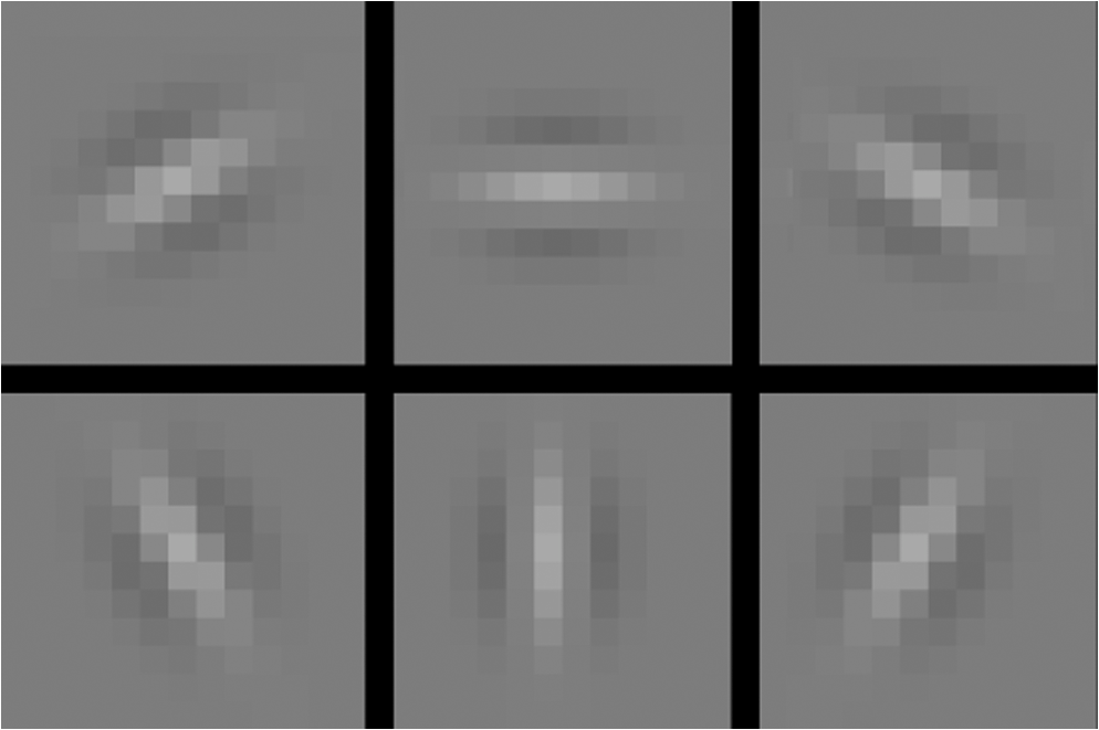
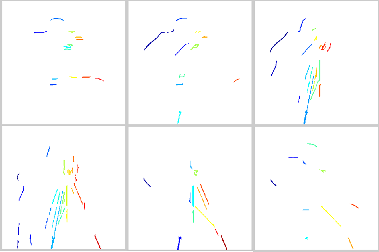
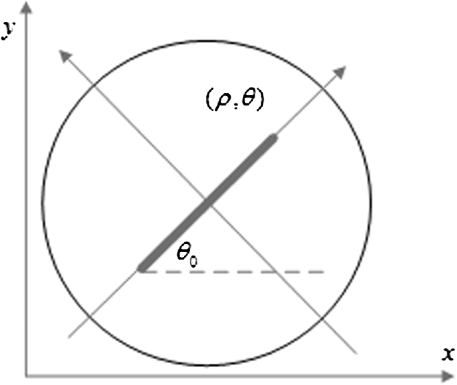
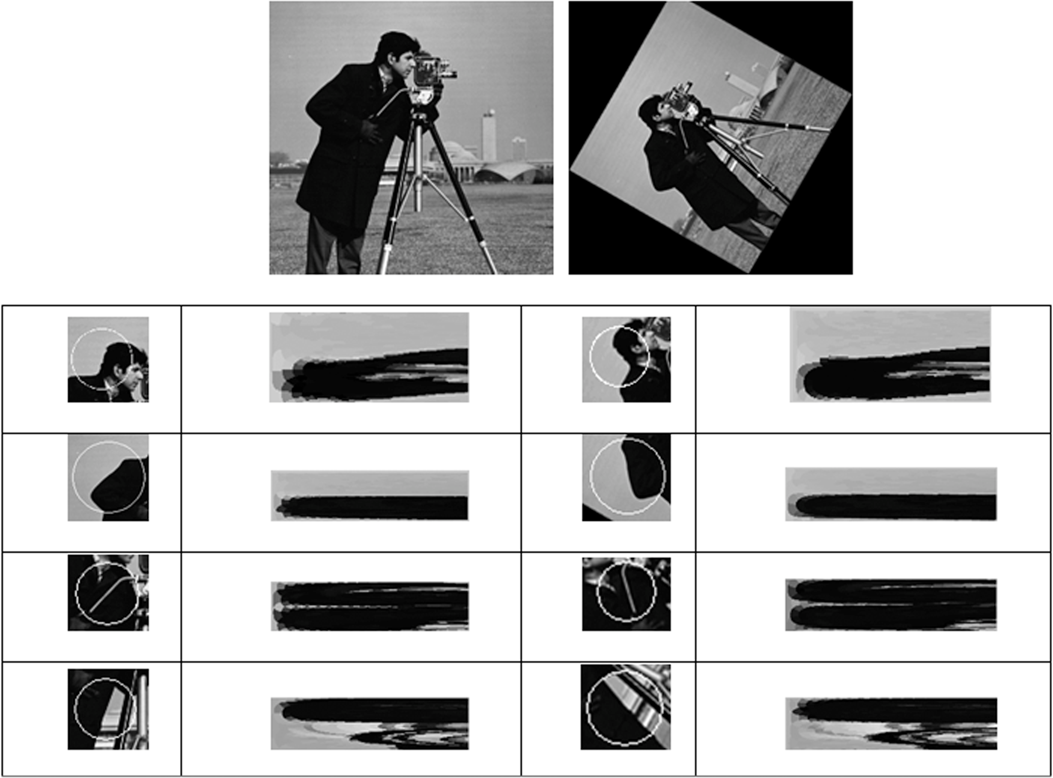
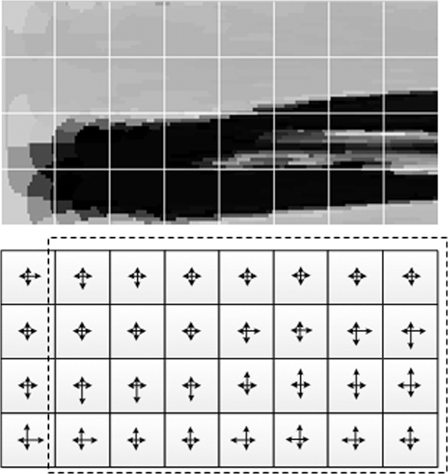
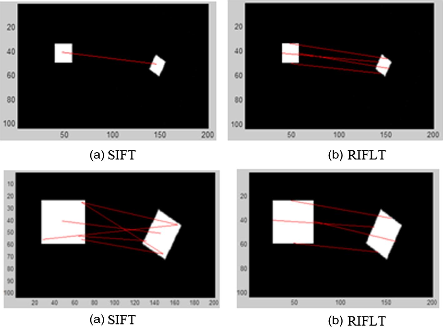
1.

Introduction

The task of finding correspondences between two images of the same scene or object, taken from different times of a day or year, different sensors, and different viewing geometries under different circumstances, is an important and difficult part of many computer vision applications. In order to match differing images, researchers have been focusing on scale and image rotation invariant detectors and descriptors.

The most widely used detector probably is the Harris corner detector, which has been proposed in 1988; Harris corners are robust to changes in rotation and intensity but are very sensitive to changes in scale, so they do not provide a good basis for matching images of different sizes. Mikolajczyk and Schmid¹ used a Harris–Laplace detector to detect the feature points in scale-space by the Laplacian-of-Gaussian operator, thus feature points are invariant to rotation and scale changes. Lowe² used a scale-invariant detector that localizes points at local scale-space maxima of the difference-of-Gaussian (DoG) in 1999, and in 2004, he presented a method called scale invariant feature transform (SIFT) for extracting distinctive invariant features from images that can be used to perform reliable matching between images.³ This approach transforms an image into a large collection of local feature vectors, each of which is invariant to image translation, scaling, rotation, and partially invariant to illumination changes and affine or three dimensional (3-D) projection. SIFT has been proven by Mikolajczyk and Schmid¹ in 2003 to be the most robust among the local invariant feature descriptors with respect to different geometrical changes.

SIFT detects feature points by searching over all scales and image locations. It is implemented efficiently by using a DoG function pyramid to identify potential interest points that are invariant to scale. By rejecting the candidate feature points that have low contrast or that are poorly localized along an edge, the dominant orientation is assigned to each feature point based on local image gradient directions. The feature descriptor is created with $4\times 4$ arrays of histograms in the neighboring region around the point, each of which has eight orientation bins, or 128 elements in sum. The matching is often based on the distance between the vectors, e.g., the Mahalanobis or Euclidean distance. Because the dimension of the descriptor and the number of the candidate key points for matching directly contribute to the time the algorithm takes, there are algorithms^4–8 that can accelerate the process by increasing the performance of descriptor of the robust features, such as speed up robust features, proposed by Bay et al.^9,10

All above descriptors are distinctive and invariant to some image transformations. The feature-based matching algorithms can be divided into three main steps. First, feature detection—for example of feature point, the interest points with the property of high repeatability are selected at distinctive locations in the image. Second, feature points description—the neighborhood of every interest point is represented by a feature vector, and there are lots of possible descriptors that emphasize a diverse set of image properties such as pixel intensity, gradient, color, texture, contour, edge, and so on. Furthermore, the descriptor has to be distinctive and robust to noise. Finally, the descriptor vectors are matched between different images. A fewer number of dimensions are therefore desirable.⁹ But the matched number of the key points cannot be too few or too many. A lack of matched key points will decrease the accuracy of matching, whereas too many will cost computational time. Because of these facts, one has to strike a balance between the above requirements, for example, by reducing the descriptor’s dimension and complexity, while keeping it sufficiently distinctive.

Figure 1 shows the SIFT matching result. There are 129 pairs of key points being matched correctly, as is shown by Fig. 1(a). However, when we add Gaussian noise with $\sigma =0.03$ to the image on the left, the number of the correct matching pairs is reduced to 26, which implies that the SIFT is somewhat sensitive to noise. In addition, the locations of the key points are concentrated.

Fig. 1

Scale invariant feature transform (SIFT) matching result.

This paper proposes a method for image matching based on feature lines rather than feature points. Kostadin et al.¹¹ has proposed a novel image denoising strategy based on an enhanced sparse representation in transform domain, by grouping similar two-dimensional image fragments into 3-D data arrays; his algorithm adapts for natural scenes. A strong similarity between small image blocks at different spatial locations is indeed very common in natural images, but our method adapts for artifices, which always contain abundant lines and clear boundaries. This paper is organized as follows: Sec. 2 describes the scheme of feature lines detection, in which distinctive feature lines with specific orientations can be detected; Sec. 3 explains polar transform of the neighborhood region of the feature lines, and a new rotation/scale invariant descriptor is also presented. Section 4 describes the matching work. Section 5 presents the experimental results, and Sec. 6 concludes the paper.

2.

Feature Lines Detection

Human vision system (HVS) includes human eyes system and human visual cortex filter system. The former can be modeled as log-polar transform, and the latter can be viewed as a range of spot and bar filters. The elementary processing method of HVS is the collected image by the human eyes system goes through the human cortex cells. These cells are not sensitive to the light of the image, but are sensitive to certain oriented structure. Thus, they are also called orientation harmonious cells, whose function, simply put, is filtering. Just like a range of spot and bar filters, some of the cortex cells respond strongly to oriented structure and weakly to other patterns. Hubel and Wiesel reason that these cortex cells function on the basis of lines or edges.¹⁰ By analogy with the human visual cortex, it is common to use at least one spot filter and a collection of oriented bar filters at different orientations, scales, and phases. After filtering, the HVS synthesizes the information resulted from all the cortex cells to make the final decision.

This work was inspired by the HVS. A new method for scene matching based on feature lines orientations, description, and matching is presented in this paper. We filter the image utilizing oriented linear Gaussian filter banks convolution to imitate the function of the cortex cells. The Gaussian filter bank has been shown in Fig. 2. Mid-grey level is represented by zero, with brighter values being positive and darker values being negative.

Fig. 2

Oriented Gaussian filters bank.

It is still unknown how many filters are “best” for useful texture algorithms. Perona listed the number of scales and orientation used in a variety of systems, ranging from 4 to 11 scales and from 2 to 18 orientations. The number of orientations varies from application to application and does not seem to make a big difference, as long as there are at least six orientations. Typically, the “spot” filters are Gaussians, and the “bar” filters are obtained by differentiating oriented Gaussians.¹² Using more filters leads to more details, but we must also convolve the image with more filters, which can be more expensive.

In this article, we utilize a range of six oriented filters; the orientations are 0, 30, 60, 90, 120, and 150 deg. There are six versions of these bars, each of which is a rotated version of a horizontal bar.

The Gaussians in the horizontal bar have weights $-1$, 2, and $-1$. They have different $\sigma$ in the $x$ and $y$ directions; the ${\sigma }_x$ values are all 2, and the ${\sigma }_y$ values are all 1. The centers are offset along the $y$ axis, lying at points (0, 1), (0, 0), and $(0,-1)$. This filters’ bank has been used by Malik and Perona in 1990.¹²

The results after applying each of the filters in Figs. 2 to 3(a) are shown in Fig. 3(b) as absolute values of the output. Brighter pixels represent stronger responses, and the images are laid out in correspondence with each of the filter position in Fig. 2.

Fig. 3

(a) Original image, (b) the responses of the filters of Fig. 2, (c) the responses of the filters under noise.

After the image is convolution filtered by the oriented linear filters, there is a strong response when the image pattern in a neighborhood looks similar to the filter kernel and a weak response when it does not, as shown in Fig. 3, and it can be hardly affected by the noise, as shown in Fig. 3(c). The advantage of this approach is that it is easy to search simple pattern elements, bars, by filtering an image. The brightness of pixels expresses responses. Then, we threshold¹³ to extract the light feature lines. The threshold value can be automatically computed by analyzing the image histogram, by obtaining the entire information contained in the histogram, the light lines with certain orientation can be extracted. Figure 4 shows the thresholding results.

Fig. 4

Extract feature lines by oriented linear Gaussian filter.

Fig. 5

Four oriented Gaussian filters bank.

Fig. 6

Extract feature lines by less linear Gaussian filter.

After automatically thresholding,^13,14 we can get six pictures with extracted feature lines by six oriented linear filters, as shown in Fig. 4.¹⁵

The number of the Oriented Gaussian filters can also be 4 as Fig. 5 shows and the extracted features lines showed in Fig. 6. One image has a range of four or six pictures of feature lines; take the feature lines in one picture as one group. If we find the correspondingly oriented pictures of the other image, the matching work will be simpler and more credible. In other words, if the approximate rotation angle of the two images could be estimated first, or one group of feature lines has been matched to another image, the matching order will be definite.

One way to estimate the approximate rotation angle of two images is using Fourier–Mellin transform (FMT).

Consider two images $f_1(x,y)$ and $f_2(x,y)$, $f_2(x,y)$ is a rotated, scaled, and translated replica of $f_1(x,y)$:

The Fourier transforms $F_1(u,v)$ and $F_2(u,v)$ of $f_1(x,y)$ and $f_2(x,y)$ are related by

Then the relation can be written as follows:

In this log-polar representation, both rotation and scaling are reduced to translations, as proposed by Pratt¹⁶ and Schalkoff.¹⁷ By Fourier transform, the log-polar representations, the rotation, and scaling appear as phase shifts. The log-polar mapping of the spectral magnitude corresponds to physical realizations of the FMT.¹⁸ Human visual systems appear to have some similarity with this log-polar mapping. The phase correlation matrix of the two transformed images is computed by

Fig. 7

Utilize Fourier–Mellin transform (FMT) to roughly estimate the rotation angle of the two images.

According to this method, we can approximately estimate the rotation angle of the two images, and the directional pictures of feature lines can be correspondingly assigned. Then, the matching work will be simpler and more credible.

But FMT is not effective for two images with big range of zooming, rotation, and transformation because FMT is a method that needs to use the whole information contained in the images. Difference in contents of two images will lead to the erroneous matching result, as is shown in Fig. 8, in which the Dirac peak has been submerged in the noises. In this condition, we should match all the six or four oriented ranges without the information of matching order.

Fig. 8

FMT cannot estimate approximate rotation angles for images with big changes.

3.

Feature Line Descriptor

Polar transform representations play an important role in image processing and analysis. In the spatial domain, log-polar schemes have been used to model the strongly inhomogeneous sampling of the retinal image by the HVS.¹⁹ Polar transform has two principal advantages: rotation invariance and scale invariance. Lines through the center of the image will be mapped into horizontal lines in the polar image and the concentric circle into vertical lines. Thus, the target rotation results in vertical translation, and the change of the target size results in horizontal translation. In other words, translating the polar image with a near edge causes the rotation of the original image. Therefore, we can transform the rotation variation to translational variation.

In order to describe the feature lines in an invariance way, we take each feature line orientation $\theta (x,y)$ as 0 deg, establish polar coordinate to transform the neighboring region of the feature line to polar image, take the feature line center as the center of the circle, and make two-thirds of the length of the feature line $r(x,y)$ as the radius, as shown in Fig. 9.

Fig. 9

Establish polar coordinate for each feature line.

For each feature line, the orientation $\theta$ and length $r$ can be computed as follows:

Because the polar coordinate takes the line orientation as the base, the polar transform is invariance to rotation angles. As the neighboring region takes the line’s length as the base, it is invariance to scaling as well. Then the circle neighboring region image is utilized to create a vector to describe the feature line. The formulas of polar transform are

Figure 10 shows the transformed polar images of the feature lines. Although the pair of feature lines has different orientations and scales, the normalized transformed polar images are almost the same.

Fig. 10

Four pairs of feature lines neighborhood transform.

4.

Local Polar Image Descriptor

The next step is to compute a descriptor for the local polar image region that is highly distinctive. One obvious approach would be to describe local polar images in a coarse-to-fine iterative strategy (pyramid approach) and to match them using a normalized correlation measure. By casting the polar image into a multiresolution framework, most of the iterations are carried out at the coarsest level, where the amount of data is greatly reduced.²⁰ This results in a considerable saving of computational time. However, simple correlation of image patches is highly sensitive to changes that may cause wrong registration of samples, such as affine or 3-D viewpoint change or nonrigid deformations.^1,21

In this article, a feature line descriptor is created by first computing the gradient magnitude and orientation at each polar image. Then, the sample points are accumulated into orientation histograms, as shown in Fig. 11. The length of each arrow corresponds to the sum of the gradient magnitudes approximating that direction within the region.

Fig. 11

Feature lines descriptor.

There are three parameters that can be chosen to vary the complexity of the descriptor: the number of orientations, $r$, in the histograms, the width, $w$, and the height $h$ of the $w\times h$ array of orientation histograms. The size of the resulting descriptor vector is $r\times w\times h$. As the complexity of the descriptor grows, it will be able to discriminate better in a large database but will also be more sensitive to shape distortions and occlusion. We can use a $4\times 8\times 4=128$ element feature vector for each feature lines, as shown in Fig. 11. As the region of the image near the center is oversampled by polar transform, there is no more information that can be used to match the left row vector that can be deleted. The eventually used number of the feature vector elements is $4\times 7\times 4=112$.

5.

Feature Line Matching

The best candidate match for each feature line is found by identifying its nearest neighbor in the database of feature lines from training images. The matching work is similar to SIFT, an effective measure is obtained by comparing the distance of the closest neighbor to that of the second-closest neighbor. Suppose there are multiple training images of the same object, the second-closest neighbor is defined as being the closest neighbor that is known to come from a different object than the first, such as by only using images known to contain different objects. This measure performs well because correct matches need to have the closest neighbor significantly closer than the closest incorrect match to achieve reliable matching. For false matches, there will likely be a number of other false matches within similar distances because of the high dimensionality of the feature space. We can consider the second-closest match as providing an estimate of the density of false matches within this portion of the feature space and at the same time identifying specific instances of feature ambiguity.¹

6.

Experiment Results and Algorithms Analysis

6.1.

Experiment Results

We coined the proposed method rotation invariant feature-line transform (RIFLT). Figure 12 shows the matching result. Figure 12(a) is the SIFT matching result, and Fig. 12(b) is the RIFLT matching result. We can see that the quantities of correct matching pairs are almost the same, but the RIFLT has two benefits: first, the RIFLT matched pairs are lines, not points; it is obvious that one line contains quite a few points; the RIFLT will contain more information. Second, because the matched feature points by SIFT are too concentrated, it is not good for image matching to compute the translation of the two images; the RIFLT feature lines are more disperse. Why the SIFT key points are so concentrated and compared with RIFLT? Does the Gaussian noise make it? Fig. 13 shows the location of the RIFLT feature lines are also disperse, compared with SIFT.

Fig. 12

Experiment results (a) utilize SIFT algorithm and (b) utilize rotation invariant feature line transform (RIFLT) algorithm proposed in this paper.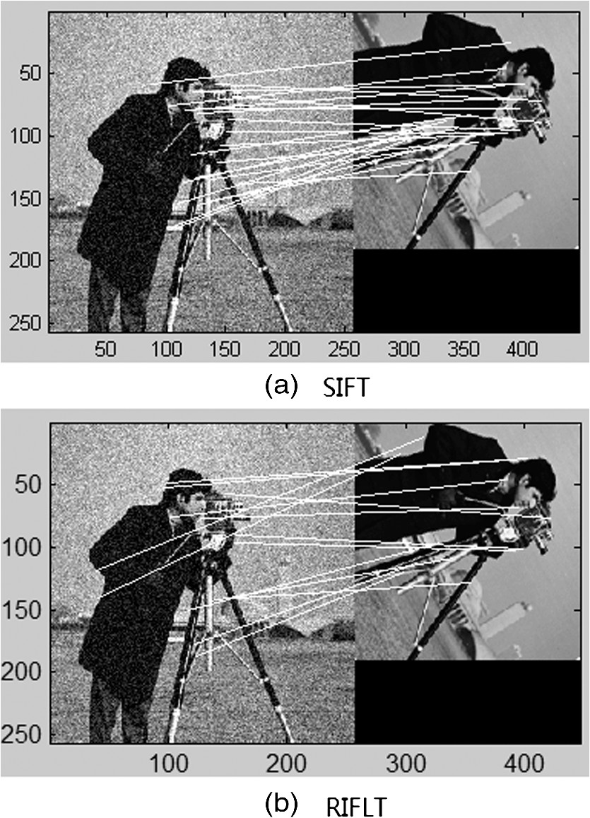

Fig. 13

Experiment results (a) utilize SIFT algorithm and (b) utilize RIFLT algorithm proposed by this paper.

We present an experiment of two simple figures, as shown in Fig. 14, one figure contains a small rectangle, and another is its rotated replica. If SIFT is utilized to match the two figures, there is only one key point, the location of the key point is in the rectangle’s center. By contrast, if RIFLT is utilized to match the two figures, there are four feature lines, the locations of the feature lines are on the edge of the rectangle. SIFT finds key points inside the change of gradients, but RIFLT find feature lines on the change of gradients, and the latter selects features that will be more disperse.

Fig. 14

(a) SIFT and (b) RIFLT for simple figure matching.

If the rectangle has been drew larger, SIFT will find more key points; the key points are under different scale spaces, but the key points are all selected by the surrounding gradient changes—the four lines. Although the quantities of the selected key points are more than the feature lines, it will make a mistake if the gradient changes are similar, as shown in Fig. 15.

Fig. 15

Experiment results (a) utilize the SIFT algorithm and (b) utilize the RIFLT algorithm proposed in this paper.

7.

Conclusions

In this paper, we present a feature line detection and description method for image matching, The feature lines have been shown to be invariant to image rotation and scale, and robust across a substantial range of affine distortion, addition of noise, and change in illumination. According to the position of the feature lines, the parameters that represent rotation angle, scaling quantity, and the transformation value can be computed. Following are the major stages of computation used to generate the set of image features:

Future work will aim at optimizing the line descriptor computation work for speed up, uniting feature points and feature lines for more robust image matching, and imitating HVS.