|
|
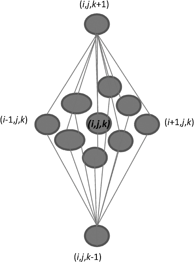
1.IntroductionThe segmentation of the brain is a task commonly developed in neuroimaging laboratories. The difficulty and importance of the skull stripping problem has led to a wide range of proposals being developed to tackle it. Some techniques reported in the literature to solve this issue are, for example, surfacing models,1 deformable models,1–3 watershed,4,5 morphology,6 atlas-based methods,7 hybrid techniques,8,9 fuzzy regions of interest,10 histogram analysis,11 active contours,12,13 multiresolution approach,14 multiatlas propagation and segmentation (MAPS),15,16 topological constraints,17 and others. Some revision papers concerning brain segmentation can be found in Refs. 1819.20.–21. The problem that arises when having many viable techniques is to choose the ones that have the best performance for a particular visualization task. In Refs. 2223.–24, the authors selected the popular skull-stripping algorithms reported in the literature and carried out a comparison among them. These algorithms include Brain Extraction Tool (BET),3 3dIntracranial,25 Hybrid Watershed Algorithm,8 Brain Surface Extractor (BSE),26 and Statistical Parametric Mapping v.2 (SPM2).27 The two common and popular methods mentioned in Refs. 22–24 are BET and BSE. According to the results presented in Ref. 23, the authors found that BET and BSE produce similar brain extractions if adequate parameters are used in those algorithms. Interesting information about BET is reported in Ref. 28, where the authors found that the BET algorithm’s performance is improved after the removal of the neck slices. Due to the popularity of BET, we will compare our results to that algorithm. Two important characteristics of BET are: it is fast and it generates approximated segmentations. In this paper, a morphological transformation that disconnects chained components is proposed and applied to segment brain from magnetic resonance imaging (MRI) T1. The operator is built as a composition between the viscous opening29 and the lower leveling30 and it is implemented in MATLAB R2010a on a 2.5 GHz Intel Core i5 processor with 2 GB RAM memory. To illustrate the performance of our proposals, two brain MRI datasets of 20 and 18 normal subjects,31 obtained from the Internet Brain Segmentation Repository (IBSR) and developed by the Centre for Morphometric Analysis (CMA) at the Massachusetts General Hospital ( http://www.nitrc.org), were processed. In order to introduce our proposals, Sec. 2 provides a background on some morphological transformations such as opening and closing by reconstruction,32 viscous opening, and lower leveling. Other approaches on viscous transformations can be found in Refs. 3334.35.–36; however, these transformations work differently because they consider structuring elements that change dynamically, while our proposals work with a geodesic approach.29 In Sec. 3, a new transformation is built through the composition of the viscous opening and the leveling. Because the composed transformation uses several parameters, a simplification of it is introduced for facilitating its application. Such a reduction results in approximated segmentations and less time is utilized during its execution. It is noteworthy to mention that the two operators employ determinate size parameters deduced from a granulometric analysis.37 The experimental results are presented in Sec. 4. In Sec. 4.1, an explanation is given about the parameters involved in the proposed transformations and the performance of each one is illustrated with several pictures. In Sec. 4.2, the results obtained with the morphological transformations are compared using the mean values of the Jaccard38 and Dice39 indices with respect to those obtained from: (i) the BET algorithm and (ii) the results reported in Refs. 11, 12, and 40, which utilize the same databases. In Sec. 4.3, the advantages and disadvantages of our method for brain MR image extraction are presented. Section 5 contains our conclusions. 2.Background on Some Morphological Transformations2.1.Opening and Closing by ReconstructionIn mathematical morphology (MM), the basic transformations are the erosion and dilation , where represents the three-dimensional (3-D) structuring element which has its origin in the center. Figure 1 illustrates the shape of the structuring element used in this paper. denotes the transposed set of with respect its origin, , is a size parameter, is the input image, and is a point on the definition domain. The next equations represent the morphological erosion and dilation :41 and where and represent the inf and sup operators. The morphological erosion and dilation permit us to build other types of transformations; these include the morphological opening and closing defined as andIn addition, the opening (closing) by reconstruction has the characteristic of modifying the regional maxima (minima) without affecting the remaining components to a large extent. These operators use the geodesic transformations.32,42 The geodesic dilation and erosion are expressed as with , and considering , respectively. When the function is equal to the morphological erosion or dilation, the opening or closing by reconstruction is obtained. Formally, the next expressions represent them and2.2.Viscous Opening and Viscous DifferenceThe viscous opening and closing defined in Ref. 29 allow one to deal with overlapped or chained components. These transformations are denoted by andEquation (2) uses three operators, the morphological erosion , the opening by reconstruction , and the morphological dilation . The morphological erosion allows one to discover and disconnect the -components (all components where the structuring element can go from one place to another by a continuous path made of squares and whose centers move along this path). Then, the opening by reconstruction removes all regions less than around the -components. Finally, because the viscous opening is defined on the lattice of dilatation, the must be obtained on . An example of Eq. (2) is given in Fig. 2. The original image is exhibited in Fig. 2(a). Figure 2(b) shows the morphological erosion . Notice that there are several components around the brain. The image in Fig. 2(c) corresponds to the transformation . In this image, several components have been eliminated by the process of opening by reconstruction. Figure 2(d) displays the result of the transformation . Viscous openings permit the sieving of the image through the viscous difference.29 This is defined in According to the explanation given above, the erosion discovers the -components and the difference with sieving the image, whereas is necessary to obtain the viscous component. The viscous difference gives the information of all discovered disconnected components of a certain size when is increased. 2.3.Lower LevelingThe lower leveling transformation is presented as follows:30 where is the reference image, is a marker, is a positive scalar called slope, and is the size of the structuring element. Equation (4) is iterated until stability is reached with the purpose of reconstructing the marker at the interior of the original mask , i.e.,On the other hand, the selection of the marker is very important. In Ref. 30, for example, the following marker was used to segment the brain: The parameter helps to control the reconstruction of the marker into . An example to illustrate the performance of Eq. (5) is given in the next section. 3.Segmentation of Brain in MRI T1Equations (2), (5), and (6) were applied in Refs. 29 and 30 to separate the skull and the brain on slices of an MRI T1 for the two-dimensional (2-D) case. These transformations allow disconnecting overlapped components, because they can control the reconstruction process. In 2-D, the structuring element moves and uniquely touches one image. However, for the 3-D case, neighbors within the structuring element are taken from three adjacent brain slices. Due to this, several regions are connected through the shape of the 3-D structuring element among the different brain sections, resulting in, as a consequence, a major connectivity. The increase in connectivity originates that Eqs. (2) and (5) for the 3-D case do not show the same performance as in the 2-D case, and the component of the brain cannot be separated by applying such operators once. This situation is illustrated in Fig. 3 where Eq. (5) has been applied considering the marker obtained by Eq. (6). The original volume appears in Fig. 3(a). Figure 3(b) displays a portion of the brain obtained from Eq. (6) with . The set of images in Figs. 3(c)–3(f) illustrates the control in the reconstruction process using different slopes . However, the extracted brain contains additional components since this condition is inadequate. The next section provides a solution to this problem. Fig. 33-D brain segmentation using Eqs. (5) and (6). (a) Original volume ; (b) marker by opening defined in Eq. (6); (c) result of Eq. (5) using the marker obtained in (b) with ; (d) result of Eq. (5) using the marker obtained in (b) with ; (e) result of Eq. (5) using the marker obtained in (b) with , and (f) result of Eq. (5) using the marker obtained in (b) with . 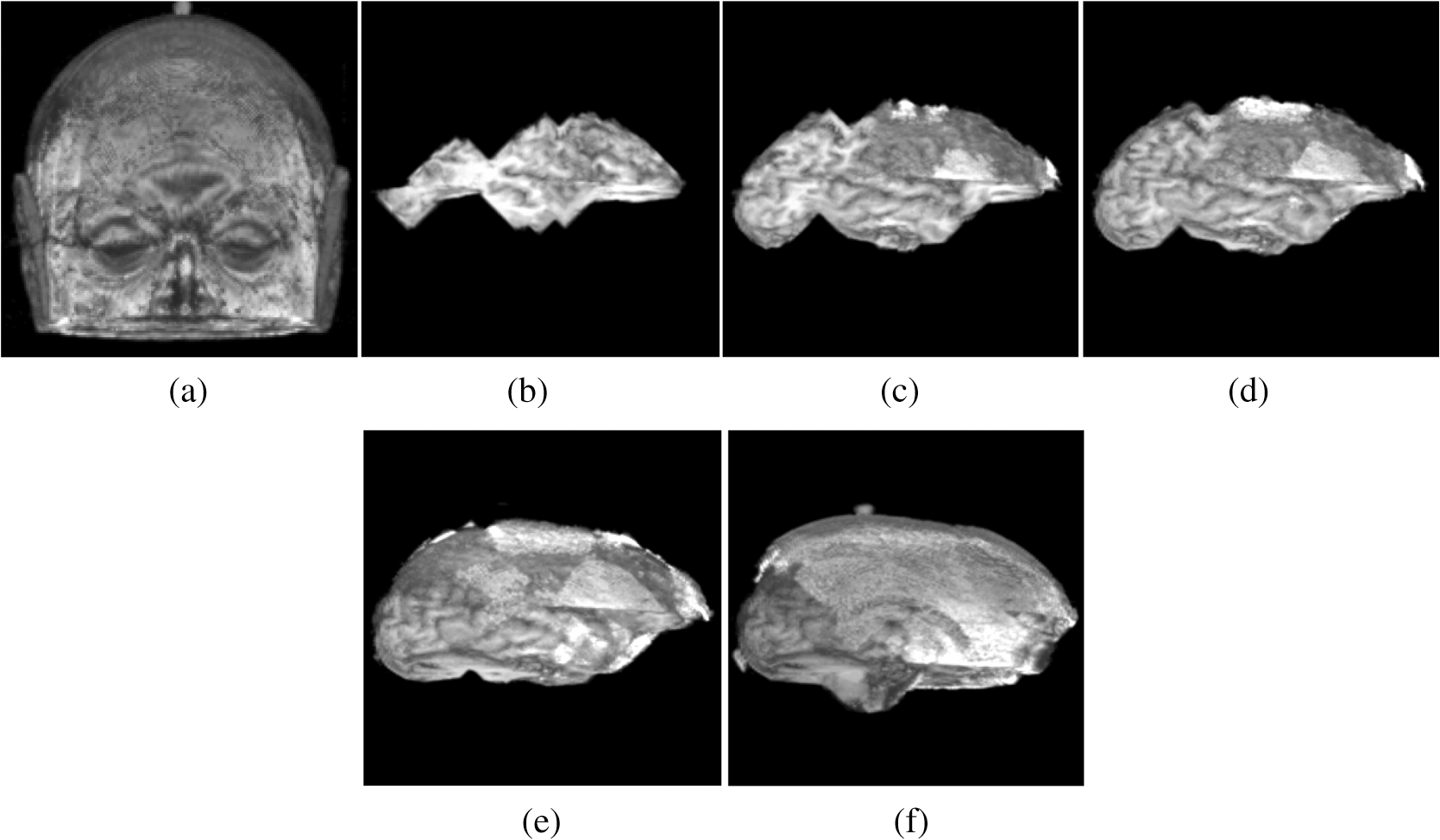 3.1.Composition of Morphological Connected TransformationsAs previously stated, viscous opening and lower leveling allow separating the chained components, and it is natural to think of combining both operators to get one transformation capable of having better control on the reconstruction process. Following this idea, an option is to use the viscous opening as a marker of the lower leveling to eliminate a great portion of the skull; posteriorly, the resulting image is again processed with a similar filter to eliminate the remaining regions around the brain. Such a procedure represents a sequential application of the combined transformations considering different parameters in order to have increasing control in the reconstruction process. The purpose is to eliminate the skull softly in two steps. The following equation permits the disconnection of the chained components and comes from the combination of Eqs. (2) and (5): Nevertheless, Eq. (7) produces an unsatisfactory performance. Figure 4 shows an example of the transformation . Some slices of the original volume can be seen in Fig. 4(a) where the segmentation results in the creation of holes on the brain, as is illustrated in Fig. 4(b). The viscous opening causes this behavior, since all components not supporting the morphological erosion of size will merge with the background because the 3-D structuring element produces stronger changes as the size of the structuring element is increased. One way to get better segmentations consists of computing the operator in Eq. (8), where is the input image, represents the mean filter of size , and expresses a threshold between sections. The mean filter partially closes the holes, and permits the selection of certain regions of interest, and helps to obtain a portion of the original image Fig. 4Segmentation of a volume [taken from the database Internet Brain Segmentation Repository (IBSR) with 20 subjects] using Eq. (7). (a) Slices of the original volume and (b) slices corresponding to .  The combination of Eqs. (7) and (8) gives the next operator as a result To apply Eq. (9), the reasoning below needs to be considered. 3.2.Parameters , , and3.2.1.ParameterThe following analysis corresponds to Eq. (5) since Eq. (9) uses it. Large values produce (i) a time reduction in reaching the final result and (ii) a larger control in the reconstruction process. The quantification of the time when Eq. (5) is applied on a volume of 60 slides—using as a marker and the lower leveling with , 3, 6, 9, 12—is presented in Fig. 5. This figure displays several slices belonging to the output volumes obtained for different values. Fig. 5Execution time of Eq. (5) and some output slices corresponding to several processed volumes. (a) Time spent to compute Eq. (5) considering 60 slices, the marker corresponds to the viscous opening with , . The leveling is applied considering , 3, 6, 9, 12; (b) graph corresponding to the data presented in (a); (c) slice of the original volume; (d) brain section taking from the viscous opening and used as marker; (e)–(i) set of slices taken from the volumes processed with , 3, 6, 9, 12, as is illustrated in Fig. 4. 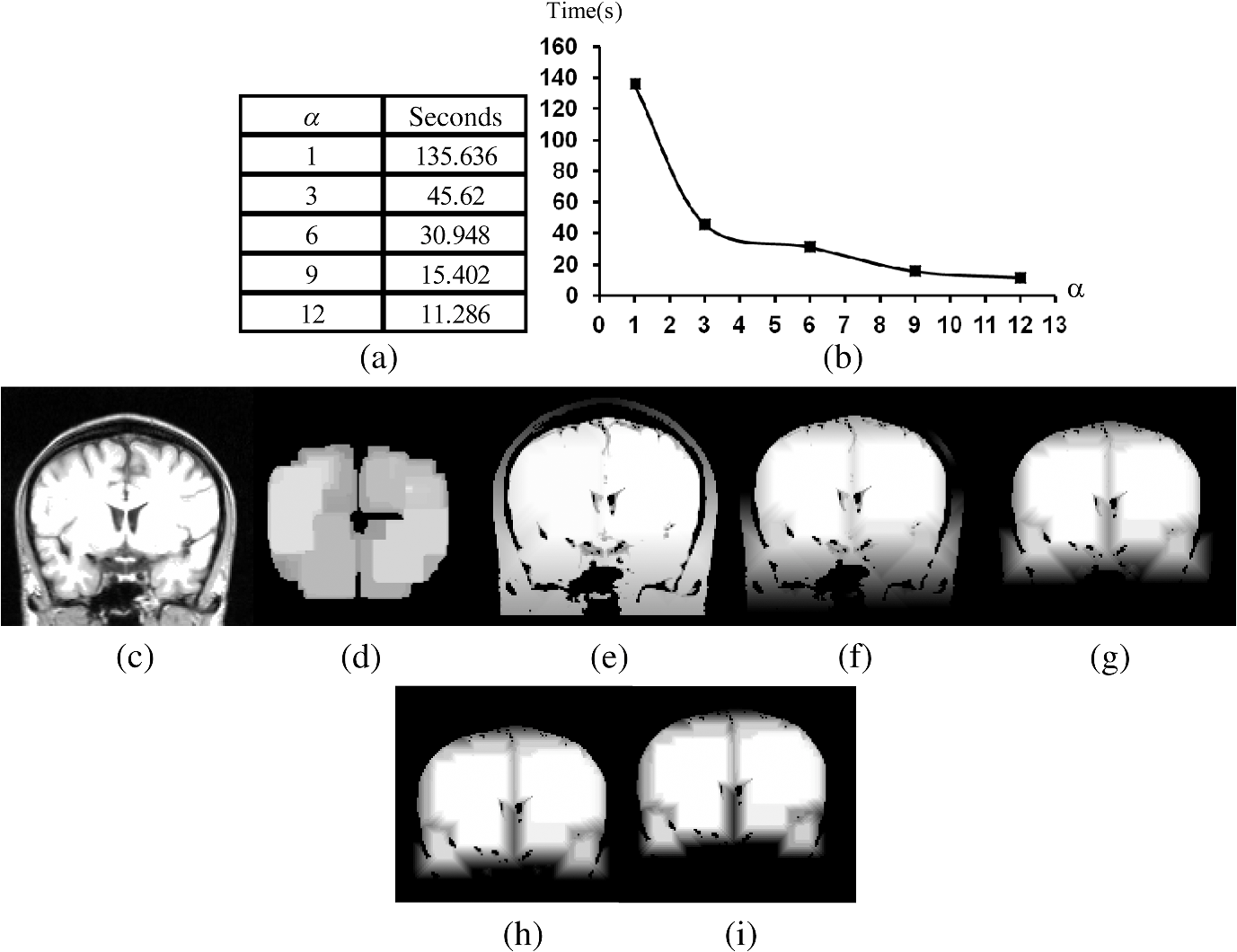 3.2.2.ParameterThe adequate election of the parameter will bring, as a consequence, the disconnection between the skull and the brain. Such a parameter is computed from a granulometric analysis applying Eq. (10)37 where vol stands for the volume, i.e., the sum of all gray levels in the image, and represents the morphological opening size . The graph in Fig. 6(a) corresponds to the application of Eq. (10) taking . This graph has three important intervals. The interval where shows the elimination of an important part of the skull. Hence, in order to detect the brain, will take values greater than 6, i.e., .3.2.3.ParameterThe parameter will be computed using the viscous granulometry which is the term of the viscous difference defined in Eq. (3)29 To apply Eq. (11), the next parameters will be considered: , , and (from the previous analysis for ), in order to detect the brain component. Figure 6(b) displays the graph of Eq. (11). For , the brain component is detected. 3.3.Simplification of Eq. (9)The fact of sequentially applying two transformations along with a mask to obtain Eq. (9) brings as a consequence the use of a large number of parameters. This problem is considered and a simplification is proposed as follows: According to Eq. (12), the marker is obtained from the viscous opening, and it is propagated by the lower leveling transformation . Equation (12) presents the following benefits when compared with respect to Eq. (9): (1) the use of fewer parameters and (2) a reduction of the execution time. The performances of Eqs. (9) and (12) are illustrated in Sec. 4. 4.Experimental ResultsFor the purpose of measuring the performance of our proposed method, the following MRI databases taken from the IBSR and developed by the CMA at the Massachusetts General Hospital ( http://www.nitrc.org)31 are utilized: (i) 20 simulated T1W MRI images (denoted as IBSR1) and (ii) 18 real T1W MRI images (denoted as IBSR2), with a slice thickness of 1.5 mm. 4.1.Parameters Involved in Eqs. (9) and (12)Tables 1Table 2Table 3–4 contain the parameters used in Eqs. (9) and (12) to segment the volumes belonging to the IBSR1 and IBSR2 datasets. In the volumes of IBSR1, the neck was cropped to obtain similar images to those of IBSR2. Differences among the volumes with respect to the intensity, size, and connectivity, originate the parameters’ variation. The guidelines for the parameter selection are given below:
Fig. 7Some brain slices corresponding to the segmentation of the volume IBSR1_100 using Eq. (9) with the parameters defined in Table 1. 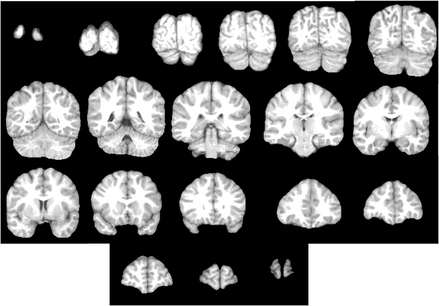 Fig. 8Some brain slices corresponding to the segmentation of the volume IBSR1_100 using Eq. (12) with the parameters defined in Table 2.  Table 1Parameters corresponding to Eq. (9). The processed dataset was IBSR1.
Table 2Parameters corresponding to Eq. (12). The processed dataset was IBSR1.
Table 3Parameters corresponding to Eq. (9). The processed dataset was IBSR2.
Table 4Parameters corresponding to Eq. (12). The processed dataset was IBSR2.
4.2.Comparison ResultsFigure 9 illustrates the resulting segmentation corresponding to the volume IBSR1_16 under the application of Eqs. (9), (12), and by BET (default parameters) implemented in the MRIcro software.43 Figure 9(a) shows the original slices. Figure 9(b) displays the respective manual segmentations. Figure 9(c) presents the application of Eq. (9) with the parameters given in Table 1. Figure 9(d) presents the application of Eq. (12) with the parameters given in Table 2. Figure 9(e) shows the brain extraction using the BET algorithm. The parameters selected for the set of 20 brains are intensity and . In order to compare the segmentations, the Jaccard and the Dice coefficients are computed. Table 5 contains the indices corresponding to BET and Eqs. (12) and (9) for the IBSR1. Fig. 9Images illustrating the segmentation of volume IBSR1_016 through several methods. (a) Brain sections corresponding to the original volume IBSR1_016; (b) manual segmentations provided by the IBSR website; (c) application of Eq. (9) with the parameters defined in Table 1; (d) application of Eq. (12) with the parameters defined in Table 2; and (e) slices obtained from BET using a and .  Table 5Jaccard and Dice indexes corresponding to IBSR1 dataset and segmented with BET, Eqs. (9) and (12) considering the parameters presented in Tables 1 and 2.
A similar procedure is applied to the IBSR2 database. Figure 10 presents the segmentations corresponding to the IBSR2_04 volume. Figure 10(a) shows the original slices. Figure 10(b) displays the respective manual segmentations. Figure 10(c) presents the application of Eq. (9) with the parameters given in Table 3. Figure 9(d) presents the application of Eq. (12) with the parameters given in Table 4. Figure 9(e) shows the brain extraction using the BET algorithm with the default parameters. Table 6 contains the Jaccard and Dice indices corresponding to BET and Eqs. (12) and (9) for the IBSR2. Fig. 10Images illustrating the segmentation of volume IBSR2_04 through several methods. (a) Brain sections corresponding to the original volume IBSR2_04; (b) manual segmentations provided by the IBSR website; (c) application of Eq. (9) with the parameters defined in Table 3; (d) application of Eq. (12) with the parameters defined in Table 4; and (e) slices obtained from BET using a and .  Table 6Jaccard and Dice indexes corresponding to IBSR2 dataset and segmented with BET, Eqs. (9) and (12) considering the parameters presented in Tables 3 and 4.
Table 7 contains the mean values of the indices presented in Tables 5 and 6 together with the mean values of the indices reported in Refs. 11, 12, and 40. Table 7Jaccard and Dice mean indexes corresponding to IBSR1 and IBSR2 datasets and some reported in the literature.
4.3.DiscussionSome commentaries on the segmented volumes are presented as follows:
5.ConclusionsTwo morphological transformations were proposed to extract brain in MRIs T1. The first operator [Eq. (9)] presents a better performance than the second one [Eq. (12)] according to the computed Jaccard and Dice mean indices. The idea to segment the brain consisted of smoothly propagating a marker given by the viscous opening into the original volume. For this, adequate parameters must be obtained from a granulometric analysis. The sequential application of such transformations results in a new morphological operator [Eq. (9)] capable of better controlling the reconstruction process. Nevertheless, the new transformation employs several parameters; due to this, a second morphological transformation was obtained from a simplification of the first one [Eq. (12)]. Our proposals were tested using the two brain databases obtained from the IBSR home page. In total, 38 volumes of MR images of the brain were processed. The segmentations were compared through two popular indices with respect to the segmentations obtained from the BET algorithm, with manual segmentations obtained from the IBSR website and with respect to the values of the indices reported in the current literature. When the mean values of the Jaccard and Dice indices are compared, our proposal outperforms the other methodologies. This means that our segmentations are closer to the manual segmentations obtained from the IBSR website. However, the time spent to segment a volume with 160 slices, along with the number of parameters utilized in Eq. (9), is higher compared to the time and the parameters utilized by the BET algorithm. Although Eq. (12) significantly reduces the number of parameters, Eq. (9) produces better segmentations. In this way, Eq. (12) can be used to get approximated segmentations of the brain. The main problem of the BET algorithm is that several regions are not detected; the beginning of Fig. 10(e) clearly illustrates this situation. Due to this, the Jaccard and Dice indices fall considerably. Finally, as future work, the proposal presented in this paper will be improved by the implementation of fast algorithms and/or parallel implementation on graphics processing units using compute unified device architectures technology, so the performance can improve for real-time applications. AcknowledgmentsThe author Iván R. Terol-Villalobos would like to thank Diego Rodrigo and Darío T.G. for their great encouragement. This work was funded by the government agency CONACyT México under the Grant 133697. ReferencesA. M. DaleB. FischlM. I. Sereno,
“Cortical surface-based analysis. I. Segmentation and surface reconstruction,”
Neuroimage, 9
(2), 179
–194
(1999). http://dx.doi.org/10.1006/nimg.1998.0395 NEIMEF 1053-8119 Google Scholar
J. X. LiuY. S. ChenL. F. Chen,
“Accurate and robust extraction of brain regions using a deformable model based on radial basis functions,”
J. Neurosci. Methods, 183
(2), 255
–266
(2009). http://dx.doi.org/10.1016/j.jneumeth.2009.05.011 JNMEDT 0165-0270 Google Scholar
S. M. Smith,
“Fast robust automated brain extraction,”
Hum. Brain Mapp., 17
(3), 143
–155
(2002). http://dx.doi.org/10.1002/(ISSN)1097-0193 HBRME7 1065-9471 Google Scholar
H. HahnH.-O. Peitgen,
“The skull stripping problem in MRI solved by a single 3D watershed transform,”
Lect. Notes Comput. Sci., 1935 134
–143
(2000). http://dx.doi.org/10.1007/b12345 LNCSD9 0302-9743 Google Scholar
R. Beareet al.,
“Brain extraction using the watershed transform from markers,”
Front. Neuroinf., 7
(32), 1
–15
(2013). http://dx.doi.org/10.3389/fninf.2013.00032 1662-5196 Google Scholar
B. DogdasD. W. ShattuckR. M. Leahy,
“Segmentation of skull and scalp in 3-D human MRI using mathematical morphology,”
Hum. Brain Mapp., 26
(4), 273
–285
(2005). http://dx.doi.org/10.1002/(ISSN)1097-0193 HBRME7 1065-9471 Google Scholar
S. SandorR. Leahy,
“Surface-based labeling of cortical anatomy using a deformable database,”
IEEE Trans. Med. Imaging, 16
(1), 41
–54
(1997). http://dx.doi.org/10.1109/42.552054 ITMID4 0278-0062 Google Scholar
F. Ségonneet al.,
“A hybrid approach to the skull stripping problem in MRI,”
Neuroimage, 22
(3), 1060
–1075
(2004). http://dx.doi.org/10.1016/j.neuroimage.2004.03.032 NEIMEF 1053-8119 Google Scholar
J. E. Iglesiaset al.,
“Robust brain extraction across datasets and comparison with publicly available methods,”
IEEE Trans. Med. Imaging, 30
(9), 1617
–1634
(2011). http://dx.doi.org/10.1109/TMI.2011.2138152 ITMID4 0278-0062 Google Scholar
F. LotteA. LecuyerB. Arnaldi,
“FuRIA: a novel feature extraction algorithm for brain-computer interfaces using inverse models and fuzzy regions of interest,”
in 3rd Int. IEEE/EMBS Conf. on Neural Engineering, 2007 (CNE ’07),
175
–178
(2007). Google Scholar
F. J. GaldamesF. JailletC. A. Perez,
“An accurate skull stripping method based on simplex meshes and histogram analysis for magnetic resonance images,”
J. Neurosci. Methods, 206
(2), 103
–119
(2012). http://dx.doi.org/10.1016/j.jneumeth.2012.02.017 JNMEDT 0165-0270 Google Scholar
S. Jianget al.,
“Brain extraction from cerebral MRI volume using a hybrid level set based active contour neighborhood model,”
Biomed. Eng. Online, 12
(1), 31
(2013). http://dx.doi.org/10.1186/1475-925X-12-31 1475-925X Google Scholar
A. Huanget al.,
“Brain extraction using geodesic active contours,”
Proc. SPIE, 6144 61444J
(2006). http://dx.doi.org/10.1117/12.654160 PSISDG 0277-786X Google Scholar
S. F. Eskildsenet al.,
“The Alzheimer’s disease neuroimaging initiative, BEaST: brain extraction based on nonlocal segmentation technique,”
Neuroimage, 59
(3), 2362
–2373
(2012). http://dx.doi.org/10.1016/j.neuroimage.2011.09.012 NEIMEF 1053-8119 Google Scholar
K. K. Leunget al.,
“Automated cross-sectional and longitudinal hippocampal volume measurement in mild cognitive impairment and Alzheimer’s disease,”
Neuroimage, 51
(4), 1345
–1359
(2010). http://dx.doi.org/10.1016/j.neuroimage.2010.03.018 NEIMEF 1053-8119 Google Scholar
K. K. Leunget al.,
“Alzheimer’s disease neuroimaging initiative, brain MAPS: an automated, accurate and robust brain extraction technique using a template library,”
Neuroimage, 55
(3), 1091
–1108
(2011). http://dx.doi.org/10.1016/j.neuroimage.2010.12.067 NEIMEF 1053-8119 Google Scholar
P. Dokládalet al.,
“Topologically controlled segmentation of 3D magnetic resonance images of the head by using morphological operators,”
Pattern Recognit., 36
(10), 2463
–2478
(2003). http://dx.doi.org/10.1016/S0031-3203(03)00118-3 PTNRA8 0031-3203 Google Scholar
M. A. Balafaret al.,
“Review of brain MRI image segmentation methods,”
Artif. Intell. Rev., 33
(3), 261
–274
(2010). http://dx.doi.org/10.1007/s10462-010-9155-0 AIREV6 0269-2821 Google Scholar
J. C. BezdekL. O. HallL. P. Clarke,
“Review of MR image segmentation techniques using pattern recognition,”
Med. Phys., 20
(4), 1033
–1048
(1993). http://dx.doi.org/10.1118/1.597000 MPHYA6 0094-2405 Google Scholar
A. P. ZijdenbosB. M. Dawant,
“Brain segmentation and white matter lesion detection in MR images,”
Crit. Rev. Biomed. Eng., 22
(5–6), 401
–465
(1994). CRBEDR 0278-940X Google Scholar
L. P. Clarkeet al.,
“MRI segmentation: methods and applications,”
J. Magn. Reson. Imaging, 13
(3), 343
–368
(1995). http://dx.doi.org/10.1016/0730-725X(94)00124-L 1053-1807 Google Scholar
C. Fennema-Notestineet al.,
“Quantitative evaluation of automated skull-stripping methods applied to contemporary and legacy images: effects of diagnosis, bias correction, and slice location,”
Hum. Brain Mapp., 27
(2), 99
–113
(2006). http://dx.doi.org/10.1002/(ISSN)1097-0193 HBRME7 1065-9471 Google Scholar
D. W. Shattucket al.,
“Online resource for validation of brain segmentation methods,”
Neuroimage, 45
(2), 431
–439
(2009). http://dx.doi.org/10.1016/j.neuroimage.2008.10.066 NEIMEF 1053-8119 Google Scholar
K. Boesenet al.,
“Quantitative comparison of four brain extraction algorithms,”
Neuroimage, 22
(3), 1255
–1261
(2004). http://dx.doi.org/10.1016/j.neuroimage.2004.03.010 NEIMEF 1053-8119 Google Scholar
B. D. Ward, Intracranial Segmentation,
(2014) http://afni.nimh.nih.gov/pub/dist/doc/program_help/ May ). 2014). Google Scholar
D. W. Shattucket al.,
“Magnetic resonance image tissue classification using a partial volume model,”
Neuroimage, 13
(5), 856
–876
(2001). http://dx.doi.org/10.1006/nimg.2000.0730 NEIMEF 1053-8119 Google Scholar
J. AshburnerK. J. Friston,
“Voxel-based morphometry: the methods,”
Neuroimage, 11
(6 Pt 1), 805
–821
(2000). http://dx.doi.org/10.1006/nimg.2000.0582 NEIMEF 1053-8119 Google Scholar
V. Popescuet al.,
“Optimizing parameter choice for FSL-Brain Extraction Tool (BET) on 3D T1 images in multiple sclerosis,”
Neuroimage, 61
(4), 1484
–1494
(2012). http://dx.doi.org/10.1016/j.neuroimage.2012.03.074 NEIMEF 1053-8119 Google Scholar
I. Santillánet al.,
“Morphological connected filtering on viscous lattices,”
J. Math. Imaging Vision, 36
(3), 254
–269
(2010). http://dx.doi.org/10.1007/s10851-009-0184-8 JIMVEC 0924-9907 Google Scholar
J. D. Mendiola-Santibañezet al.,
“Application of morphological connected openings and levelings on magnetic resonance images of the brain,”
Int. J. Imaging Syst. Technol., 21
(4), 336
–348
(2011). http://dx.doi.org/10.1002/ima.v21.4 IJITEG 0899-9457 Google Scholar
Center for Morphometric Analysis, Massachusetts General Hospital, The Internet Brain Segmentation Repository (IBSR) (
(1995) http://www.cma.mgh.harvard.edu/ibsr/ May 2014). Google Scholar
L. Vincent,
“Morphological grayscale reconstruction in image analysis: applications and efficient algorithms,”
IEEE Trans. Image Process., 2
(2), 176
–201
(1993). http://dx.doi.org/10.1109/83.217222 IIPRE4 1057-7149 Google Scholar
F. MeyerC. Vachier,
“Image segmentation based on viscous flooding simulation,”
Mathematical Morphology, 69
–77 CSIRO Publishing, Melbourne
(2002). Google Scholar
C. VachierF. Meyer,
“The viscous watershed transform,”
J. Math. Imaging Vis., 22
(2–3), 251
–267
(2005). http://dx.doi.org/10.1007/s10851-005-4893-3 JIMVEC 0924-9907 Google Scholar
P. MaragosC. Vachier,
“A PDE formulation for viscous morphological operators with extensions to intensity-adaptative operators,”
in Proc. 15th IEEE Int. Conf. in Image Processing,
2200
–2203
(2008). Google Scholar
C. VachierF. Meyer,
“News from viscous land,”
in Proc. of the 8th Int. Symposium on Mathematical Morphology,
189
–200
(2007). Google Scholar
L. Vincent,
“Fast granulometric methods for the extraction of global image information,”
in Proc. 11th Annual Symposium of the South African Pattern Recognition Association,
119
–133
(2000). Google Scholar
P. Jaccard,
“The distribution of the flora in the alpine zone,”
New Phytol., 11
(2), 37
–50
(1912). http://dx.doi.org/10.1111/nph.1912.11.issue-2 NEPHAV 0028-646X Google Scholar
L. R. Dice,
“Measures of the amount of ecologic association between species,”
J. Ecol., 26
(4), 297
–302
(1945). http://dx.doi.org/10.2307/1932409 JECOAB 0022-0477 Google Scholar
H. Zhanget al.,
“An automated and simple method for brain MR image extraction,”
Biomed. Eng. Online, 10
(1), 81
(2011). http://dx.doi.org/10.1186/1475-925X-10-81 1475-925X Google Scholar
H. Heijmans, Morphological Image Operators, Academic Press, Boston, Massachusetts
(1994). Google Scholar
J. SerraP. Salembier,
“Connected operator and pyramids,”
Proc. SPIE, 2030 65
–76
(1993). http://dx.doi.org/10.1117/12.146672 PSISDG 0277-786X Google Scholar
C. RordenM. Brett,
“Stereotaxic display of brain lesions,”
Behav. Neurol., 12
(4), 191
–200
(2000). http://dx.doi.org/10.1155/2000/421719 BNEUEI 0953-4180 Google Scholar
BiographyJorge Domingo Mendiola-Santibañez received his PhD degree from the Universidad Autónoma de Querétaro (UAQ), México. Currently, he is a professor/researcher at the Universidad Autónoma de Querétaro. His research interests include morphological image processing and computer vision. Martín Gallegos-Duarte is an MD and a PhD student at the Universidad Autonoma de Querétaro. He is head of the Strabismus Service at the Institute for the Attention of Congenital Diseases and Ophthalmology-Pediatric Service in the Mexican Institute of Ophthalmology in the state of Queretaro, Mexico. Miguel Octavio Arias-Estrada is a researcher in computer science at National Institute of Astrophysics, Optics and Electronics, Puebla, Mexico, with a PhD degree in electrical engineering (computer vision) from Laval University (Canada) and BEng and MEng degrees in electronic engineering from University of Guanajuato (Mexico). Currently, he is a researcher at INAOE (Puebla, México). His interests are computer vision, FPGA and GPU algorithm acceleration for three-dimensional machine vision. Israel Marcos Santillán-Méndez received the BS degree in engineering from the Instituto Tecnológico de Estudios Superiores de Monterrey and his MS degree and PhD degree in engineering from Facultad de Ingeniería de la Universidad Autónoma de Querétaro (México). His research interests include models of biological sensory and perceptual systems and mathematical morphology. Juvenal Rodríguez-Reséndiz received his MS degree in automation control from University of Querétaro and PhD degree at the same institution. Since 2004, he has been part of the Mechatronics Department at the UAQ. He is the head of the Automation Department. His research interest includes signal processing and motion control. He serves as vice president of IEEE in Queretaro State. Iván Ramón Terol-Villalobos received his BSc degree from Instituto Politécnico Nacional (I.P.N. México), his MSc degree from Centro de Investigación y Estudios Avanzados del I.P.N. (México). He received his PhD degree from the Centre de Morphologie Mathématique, Ecole des Mines de Paris (France). Currently, he is a researcher at CIDETEQ (Querétaro, México). His main current research interests include morphological image processing, morphological probabilistic models, and computer vision. |
|||||||||||||||||||||||||||||||||||||||||||||||||||||||||||||||||||||||||||||||||||||||||||||||||||||||||||||||||||||||||||||||||||||||||||||||||||||||||||||||||||||||||||||||||||||||||||||||||||||||||||||||||||||||||||||||||||||||||||||||||||||||||||||||||||||||||||||||||||||||||||||||||||||||||||||||||||||||||||||||||||||||||||||||||||||||||||||||||||||||||||||||||||||||||||||||||||||||||||||||||||||||||||||||||||||||||||||||||||||||||||||||||||||||||||||||||||||||||||||||||||||||||||||||||||||||||||||||||||||||||||||||||||||||||||||||||||||||||||||||||||||||||||||||||||||||||||||||||||||||||||||||||||||||||||||||||||||||||||||||||||||||||||||||||||||||||||||||||||||||||||||||||||||||||||||||||||||||||||||||||||||||||||||||||||||||||||||||||||||||||||||||||||||||||||||||||||||||||||||||||||||||||||||||||||||||||||||||||||||||||||||||||||||||||||||||||||||||||||||||||||||||||||||||||||||||||||||||||||||||||||||||||||||||||||||||||||||||||||||||||||||||||||||||||||||||||||||||||||||||