Morphological segmentation approaches of directional structures based on connections

Carlos A. Paredes-Orta; Jorge D. Mendiola-Santibanez; Ana M. Herrera-Navarro; Luis A. Morales-Hernandez; Ivan Terol-Villalobos

doi:10.1117/1.JEI.23.2.023007

17 March 2014 Morphological segmentation approaches of directional structures based on connections

Carlos A. Paredes-Orta, Jorge D. Mendiola-Santibanez, Ana M. Herrera-Navarro, Luis A. Morales-Hernandez, Ivan Terol-Villalobos

Author Affiliations +

Journal of Electronic Imaging, Vol. 23, Issue 2, 023007 (March 2014). https://doi.org/10.1117/1.JEI.23.2.023007

Abstract

The multiscale morphological approaches for segmenting directional structures are proposed. First, the use of the composition of connections to extract the directional structures of the image is investigated. We show that even though the composition of connectivities enables the correct determination of the main directional structures, the requirement of the scales for segmenting the image makes this algorithm more or less complex to apply. Then, a morphological image segmentation approach is proposed based on the concept of connectivity in a viscous lattice sense. Two functions are computed to characterize the directional structures: viscosity and orientation. The viscosity function codifies the different scales of the structure and is computed from the supremum of directional erosions. This function contains the sizes of the longest lines that can be included in the structure. To determine the directions of the line segments, the orientation function is employed. By combining both images—viscosity and orientation functions— an orientation partition function is created. This last function contains information of the maxima of the viscosity function and their orientation. Finally, the elements of the orientation partition function are merged according to some criteria, using a histogram-based segmentation approach to compute an optimal partition.

1. Introduction

Although anisotropic structures are frequently found in many classes of images (materials, biometry images, biology, remote sensing, among others), few works dealing with directional analysis in morphological image processing have been carried out. There are some studies that treat this subject from an algorithmic point of view,¹^,² while application analysis has been addressed elsewhere.³^–²² Among these works, the most interesting is that proposed by Soille and Talbot,¹ in which the authors carry out a comprehensive study on directional morphological filtering. Despite the numerous applications of anisotropic structures, it is in the domain of fingerprint recognition [see Fig. 1(a)], which is the most widely used biometric features for personal identification today, where the study of directional structures based on field-orientation detection is an active subject of research. Some recent papers on this subject are Refs. 5 and 8 to 13, just to mention a few. In particular, the work of Oliveira and Leite⁵ is of great interest since there are only few works in the literature that characterize fingerprints based on mathematical morphology.

Fig. 1

Examples of directional structures. (a) Fingerprint image. (b) Pearlitic phase image. (c) and (d) Segmented images.

However, orientation detection also plays a fundamental role in other domains.¹⁴^–²² Lee et al.¹⁴ proposed a method based on oriented connectivity for segmenting solar loops, while Kass and Witkin¹⁶ introduced a method to analyze oriented patterns in wood grain. On the other hand, a new approach has been introduced by Sandberg and Brega¹⁷ for segmenting thin structures in electron micrographs. Recently, Truc et al.¹⁹ proposed a vessel enhancement framework for angiography images based on directional filter bank, whereas Wang and Tseng²⁰ introduced an adaptive dual-directional filter based on a slope filter. This last work is focused on the filtering of nonground points from point clouds to obtain terrain relief from airborne LiDAR data. Also, directional filtering has been used to remove noise.²¹^,²² In addition, the orientation may play a fundamental role to characterize structures in materials science.³^,²³^,²⁴ For example, the pearlite phase displays a morphology in the form of parallel lines [see Fig. 1(b)], and when further grains are formed, these can change direction. In this case, the extraction of directional structures from an image becomes a useful technique. It is well known that many physical and mechanical properties in materials are closely related to microstructure. Thus, great interest exists in the use of image-processing techniques for determining the relationship between microstructure and material properties.

Given the interest in orientation pattern models for characterizing structures, this paper investigates the use of mathematical morphology for modeling orientation structures. In particular, we focus on the problem of segmenting images containing directional structures as those shown in Fig. 1. As in the human vision system, computer image processing of oriented image structures often requires a bank of directional filters or template masks, each of them sensitive to a specific range of orientations. Hence, one investigates the use of a bank of filters based on directional morphology. Particularly, we will focus on the most sensitive filters that can detect the critical elements of the structure. In the literature, several works characterize directional structures based on the computation of gradients, which can be formalized in terms of mathematical morphology. See, for example, Refs. 9, 16, and 18. The problem with gradients is that they work at pixel scale; they are very sensitive to noise and a final stage is required to enhance directional structures. Therefore, the main idea in this paper is motivated by another approach that permits to take into account the whole context of the structures contained in an image. Mainly, two methods for segmenting directional structures are introduced. First, a segmentation method based on a composition of connections generated by openings and dilations using directional structuring elements is introduced. This method enables the correct segmention of this type of structures. The major drawback of this approach is the number of parameters that must be taken into account. Second, to decrease the complexity, an approach based on directional erosions, which takes into account the connectivity in the viscous lattice sense, is proposed. Strictly speaking, this last method requires only one parameter that is linked to the number of regions of the segmented image.

This paper is organized as follows. In Sec. 2, the concepts of morphological filter, directional morphology, and the connected class notion are presented. In Sec. 3, a method for segmenting images based on a composition of connections is introduced. Subsequently, in Sec. 4, the notions of viscosity and orientation functions derived from the supremum of directional erosions are proposed. Also, an algorithm for segmenting the images based on the notion of the orientation partition function (OPF) and the histogram of orientations is proposed. The OPF is built using the viscosity function, the orientation function, and the catchment basins transformation. The proposed algorithms are discussed in Sec. 5, and the limits of the approach are addressed as well.

2. Some Basic Concepts of Morphological Filtering and Connections

2.1.

Basic Notions of Morphological Filtering

Mathematical morphology is mainly based on the so-called increasing transformations.²⁵^–²⁷ A transformation $T$ is increasing if for two sets $X$ , $Y$ such that $X \subset Y \Rightarrow T (X) \subset T (Y)$ . In the gray-level case, the inclusion is substituted by the usual order, i.e., let $f$ and $g$ be two functions; then $f \leq g \Leftrightarrow f (x) \leq g (x)$ for all $x$ . Then, a transformation $T$ is increasing if for all pair of functions $f$ and $g$ , with $f \leq g \Leftrightarrow T (f) \leq T (g)$ . In other words, increasing transformations preserve the order. A second important property is the idempotence notion. A transformation $T$ is idempotent if and only if $T T [(f)] = T (f)$ . The use of both properties plays a fundamental role in the theory of morphological filtering. In fact, one calls morphological filter to all increasing and idempotent transformations. The basic morphological filters are the morphological opening $γ_{λ B}$ and the morphological closing $φ_{λ B}$ with a given structuring element. Here, $B$ represents the elementary structuring element containing its origin (for example, a square of $3 \times 3 pixels$ ), $\overset{˘}{B}$ is the transposed set ( $\overset{˘}{B} = {- x : x \in B}$ ), and $λ$ is a homothetic parameter. Then, the morphological opening and closing are given by

Eq. (1)

γ_{λ B} (f) = δ_{λ \overset{˘}{B}} [ε_{λ B} (f)] and φ_{λ B} (f) = ε_{λ \overset{˘}{B}} [δ_{λ B} (f)],

where the morphological erosion

ε_{λ B}

and dilation

δ_{λ B}

are expressed by

ε_{λ B} (f) (x) = \land {f (y) : y \in λ {\overset{˘}{B}}_{x}}

and

δ_{λ B} (f) (x) = \lor {f (y) : y \in λ {\overset{˘}{B}}_{x}}

, respectively, and

\land

is the inf operator and

\lor

is the sup operator. Henceforth, the set

B

will be suppressed, so the expressions

γ_{μ}

and

γ_{μ B}

are equivalent (

γ_{μ} = γ_{μ B}

). When the parameter

μ

is equal to one, all parameters are suppressed (

δ_{B} = δ

).

In the present work, we are particularly interested in morphological directional transformations that are characterized by two parameters. A directional structuring element depends on its length (size $λ$ ) and the slope (angle $α$ ) of the element. Thus, the set of points of a line structuring element $L_{α, λ}$ is computed by two sets of points for $α \in [0, 90]$ . These sets of points ${(x_{i}, y_{i})}$ are defined by the following expressions:

if 0 \leq α \leq 45 then, y_{i} = x_{i} \tan (α) for x_{i} = 0, 1, \dots, (λ / 2) \cos (α) if 90 \geq α > 45 then, x_{i} = y_{i} \cot (α) for y_{i} = 0, 1, \dots, (λ / 2) \cos (α)

and the set of points

{(- x_{i}, - y_{i})}

. This means that the structuring element is a symmetric set. Similar expressions can be found for

α \in (90,180]

. Then, the morphological opening and closing are given by

Eq. (2)

γ_{α, λ} (f) = δ_{α, λ} [ε_{α, λ} (f)] and φ_{α, λ} (f) = ε_{α, λ} [δ_{α, λ} (f)],

where the morphological erosion and dilation are given by

ε_{α, λ} (f) (x) = \land_{}^{} {f (y) : y \in L_{α, λ} (x)}

and

δ_{α, λ} (f) (x) = \lor_{}^{} {f (y) : y \in L_{α, λ} (x)}

.

2.2.

Connected Classes

One of the most interesting concepts proposed in mathematical morphology is the notion of connected classes introduced by Serra.²⁵ Intensive work has been done on the study of connectivity classes. Recent studies dealing with this subject have been carried out in Refs. 28 29.30.31.32.33.34.35.36.37. to 38. In fact, a connection or connected class on $E$ is a set family $C \subseteq P (E)$ that satisfies the following three axioms:

i/ $\emptyset \in C$ ,
ii/ $x \in E \Rightarrow {x} \in C$ ,
iii/ for each family $X_{i}$ in $C$ , $\cap X_{i} \neq \emptyset \Rightarrow \cup X_{i} \in C$ .

An equivalent definition to the connected class is the connection openings expressed by the following theorem, which provides an operating way to act on connections.

Theorem 1 (Connection openings)

The datum of a connected class $C$ on $P (E)$ is equivalent to the family ${γ_{x}, x \in E}$ of the so-called connection openings such that

i/ for all $x \in E$ , we have $γ_{x} (x) = {x}$ ,
ii/ for all $A \subseteq E$ , $x, y$ in $E$ , $γ_{x} (A)$ and $γ_{y} (A)$ are equal or disjoint,
iii/ for all $A \subseteq E$ and for all $x \in E$ , we have $x \notin A \Rightarrow γ_{x} (A) = \emptyset$ .

Observe that $γ_{x} (A)$ , $x \in E$ constitutes a partition of $A$ . In the present work, we will focus on three connections: connections generated by extensive dilations and openings, and the connection on viscous lattices.

The first one, based on extensive dilations, acts by clustering the arc-wise connected components.²⁵^,²⁹

Definition 1.

Let $γ_{x}$ , $x \in E$ , be a system of connectivity openings on $P (E)$ corresponding to a connectivity class $C$ . For each $x \in E$ , define the operator $ν_{x}$ on $P (E)$ by

Eq. (3)

ν_{x} (X) = X \cap γ_{x} δ_{λ} (X) .

Another connection³¹ is given by the openings as follows.

Definition 2.

Let $C$ be a connectivity class and $γ_{λ}$ an opening on $P (E)$ . Let $C_{σ}$ be the subset of $C$ consisting of $\emptyset$ , all singletons ${x}$ , and all elements of $C \cap Inv (γ)$ . Then, $C_{σ}$ is a connectivity class with associated connectivity openings given by

Eq. (4)

σ_{x} (X) = {\begin{cases} γ_{x} γ_{λ} (X), & if x \in γ_{λ} (X) \\ x, & if x \in X ∖ γ_{λ} (X) \\ \emptyset, & if x \notin X \end{cases} .

Then, $C_{σ}$ is a connection on $P (E)$ , and for any $X \in P (E)$ , the connected components according to $C_{σ}$ are the connected components of $γ_{λ} (X)$ and the singletons of $X ∖ γ_{λ} (X)$ . Finally, let us introduce the connection on viscous lattices.³⁵^,³⁹ In Ref. 35, the usual space $P (E)$ is replaced by a viscous lattice structure given by the family $L = {δ_{λ} (X), X \in P (E)}$ ; with $λ > 0$ , that is both the image $P (E)$ under an extensive dilation $δ_{λ}$ and under the opening $δ_{λ} ε_{λ}$ . Now, let $C$ be a connected class on $P (E)$ . Since dilation $δ_{λ}$ is extensive by definition, it preserves the whole class $C$ , and the adjoint erosion $ε_{λ}$ treats the connected component independent of each other, i.e., $X = \cup {X_{i}, X_{i} \in C} \Rightarrow ε_{λ} (X) = \cup ε_{λ} (X_{i})$ .

Given that Serra proposes to define connections on $P (E)$ before the dilation $δ_{λ}$ , thus, one expresses the $C'$ viscous connected components of a given set $A$ as a function of its $C$ components (arc-wise connected components) as

Eq. (5)

γ_{δ (x)} = δ_{λ} γ_{x} ε_{λ} .

According to this proposition, the number of connected components depends on the viscosity parameter $λ$ . Figure 2(a) illustrates the original image composed of three arc-wise connected components or three components at viscosity $λ = 0$ . Figures 2(b) to 2(e) show the eroded images by disks of sizes 20, 22, 27, and 36, respectively. Then, at viscosity $λ = 20$ , one has four connected components, whereas at viscosity $λ = 22$ , the image is composed of five connected components [see Figs. 2(b) and 2(c)]. The image in Fig. 2(f) shows the connected components for viscosity $λ = 22$ . However, by considering disks as the elementary shapes of the image, it is not possible to detect six connected components for any viscosity. The solution to this problem is to select the connected components at different viscosities (scales). The traditional algorithm is the well-known ultimate erosion, and it consists of selecting the connected components at viscosity $λ$ such that they are removed for viscosity $λ + 1$ . Another way to select the connected components is to compute the distance function as shown in Fig. 2(g) and detect its maxima. The image in Fig. 2(h) shows the ultimate eroded components for viscosities (sizes) 25, 34, 45, 64, 66, and 68, whereas Fig. 2(i) illustrates the connected components in the viscous lattice sense. This is a most interesting connection since it exploits the goal in binary image segmentation, which is to split the connected components into a set of elementary shapes.

Fig. 2

Viscous connectivity. (a) Original image $X$ (b), (c), (d), and (e) Eroded connected components at viscosity $λ = 20$ , $λ = 22$ , $λ = 27$ , and $λ = 36$ , respectively. (f) Connected components at viscosity $λ = 22$ ,. (g) Distance function. (h) Maxima of distance function (ultimate eroded). (i) Connected components in the viscous lattice sense computed from the maxima. (j) Segmentation by watershed. (k) Connected components.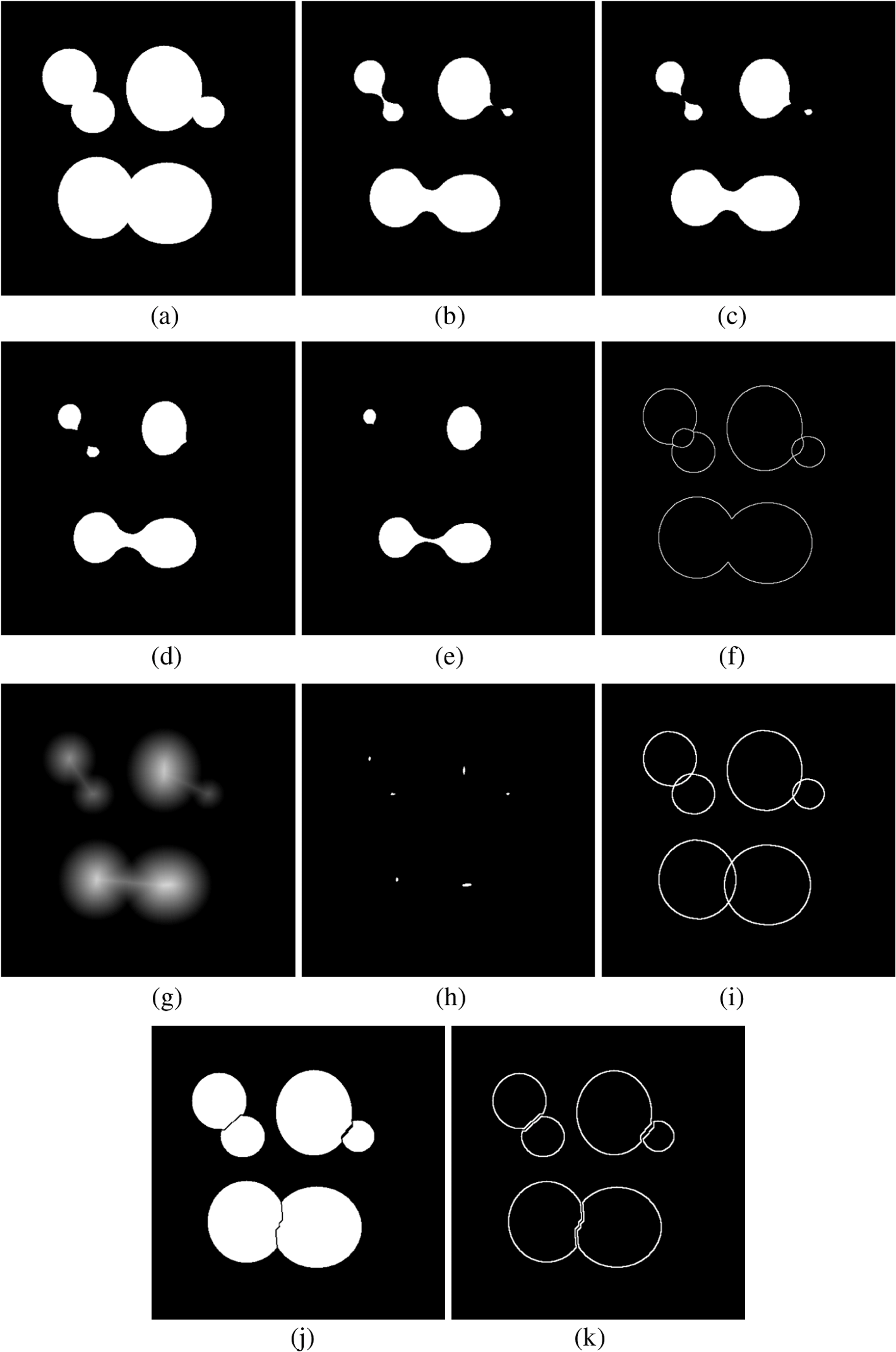

3. Image Segmentation of Directional Structures Based on a Composition of Connections: Connectivities Generated by Openings and Dilations

Image segmentation is one of the most interesting problems in mathematical morphology.⁴⁰^–⁴² It is well-known that the notion of connectivity is linked to the intuitive idea of a segmentation task, where the objective is to determine a set of elementary shapes (connected components) that will be processed separately. The result of the segmentation depends on the notion of connected components. If one supposes a priori that the elementary shapes of the set in Fig. 2(a) are disks, then the viscous connection gives better results than the watershed transformation [see Figs. 2(j) and 2(k)]. Similarly, for the images shown in Fig. 1, the problem lies in determining what a connected component is. Different approaches can be chosen to introduce such a concept based on the connected classes notion. According to the usual connectivity, the set $X$ in Fig. 3(a) is composed of 13 connected components. However, the number of connected components of this set depends on the connection used to analyze it. For example, using the connection generated by openings $C_{σ}$ [Eq. (4)], the connected components of the set $X$ are given by all singletons ${x} \in X ∖ γ_{α, λ} (X)$ and all elements of $γ_{α, λ} (X)$ . Nevertheless, from a practical point of view, the use of a partial connection of $C_{σ}$ is more interesting as proposed by Ronse.³² In this case, for the partial connection $C_{σ}^{*}$ , the connected components of a set $X$ are the connected components of $γ_{λ} (X)$ , whereas $X ∖ γ_{λ} (X)$ will be the residual. Then, by using the partial connection $C_{σ}^{*}$ , this set can be interpreted differently. Consider three-directional openings with $λ_{1} = 25$ and $α_{1} = {45,90,135}$ and the derived partial connection openings given by

Eq. (6)

σ_{x}^{γ_{α_{1}, λ_{1}}} (X) = {\begin{cases} γ_{x} γ_{α_{1}, λ_{1}} (X), & if x \in γ_{α_{1}, λ_{1}} (X) \\ \emptyset, & if x \notin γ_{α_{1}, λ_{1}} (X) \end{cases} .

Fig. 3

Composition of connections. (a) Original image $X$ ,. (b), (c), and (d) Connected components according to $\underset{x}{V} σ_{x}^{γ_{90, 25}} (X)$ , $\underset{x}{V} σ_{x}^{γ_{45, 25}} (X)$ and $\underset{x}{V} σ_{x}^{γ_{135, 25}} (X)$ , respectively. (e), (f), and (g) Connected components according to $\underset{y}{V} κ_{y}^{90, 25, 0, 15} (X)$ , $\underset{y}{V} κ_{y}^{45,25,135, 15} (X)$ and $\underset{y}{V} κ_{y}^{135, 25, 45, 15} (X)$ , respectively. (h) Connected components according to the composed connectivity.

For $α_{1} = 90$ , the original image has 17 connected components as illustrated in Fig. 3(b), whereas for $α_{1} = 45$ , the image $X$ is composed of 13 connected components as shown in Fig. 3(c). Finally, for $α_{1} = 135$ , there also exist 13 connected components as illustrated in Fig. 3(d). Nevertheless, from a practical point of view [see Figs. 1(c) and (d)], the connected components according to $C_{σ}^{*}$ , must be analyzed by a clustering process derived from the connection $C_{ν}$ in Definition 1. One requires a connectivity generated by the composition of the partial connection $C_{σ}^{*}$ and the connection $C_{ν}$ . Thus, the connected components are given by

Eq. (7)

κ_{y}^{α_{1}, λ_{1}, α_{2}, λ_{2}} (X) = ν_{y}^{δ_{α_{2}, λ_{2}}} [V_{x} σ_{x}^{γ_{α_{1}, λ_{1}}} (X)] = ν_{y}^{δ_{α_{2}, λ_{2}}} [γ_{α_{1}, λ_{1}} (X)] .

By using directional dilations with parameters $λ_{2} = 15$ and $α_{2} \in {0,135, 45}$ applied to Figs. 3(b) to 3(d), respectively, one computes the images in Figs. 3(e) to 3(g). According to this composed connection, the set $X$ has five connected components for $V_{y} κ_{y}^{90, 25, 0, 15} (X)$ , $V_{y} κ_{y}^{45,25,135, 15} (X)$ , and $V_{y} κ_{y}^{135, 25, 45, 15} (X)$ as illustrated in Figs. 3(e) to 3(g). Then, the set $X$ has 15 connected components as shown in Fig. 3(h).

In the real case, see Figs. 1(a) and 1(b), the task of extracting the connected components becomes a difficult problem since they are not well separated and belong to different scales (see Fig. 4). For example, the composed connection using two-directional openings of size $λ_{1} = 20$ and $α_{1} = {45, 60}$ and directional dilations using $λ_{2} = 10$ and $α_{2} = {135,150}$ were applied to the image in Fig. 4(a). Then, the largest connected components, illustrated in Figs. 4(b) and 4(c), were extracted according to $κ_{y}^{45,20,135, 10}$ and $κ_{y}^{60,20,150, 10}$ . Now, the main problem lies in deciding which of these connected components represents a region better in the original image. A simple criterion to take this decision is to choose the largest one. Thus, the solution to extract the largest connected component from the set $X$ lies in applying to this set the $κ$ operator with fixed size parameters $λ_{1}$ and $λ_{2}$ , $α_{1} \in [0,180]$ and $α_{2}$ perpendicular to $α_{1}$ . Then, one must take the largest connected component $A_{1}$ for all $α_{1}$ . As a precision, when the operator $ν_{y}^{δ_{α_{2}, λ_{2}}}$ is applied, it is preferable to make the intersection with the original image. Figure 4(d) illustrates this component. Next, one computes the residual $X ∖ A_{1}$ as shown in Fig. 4(e), and the operator $κ$ is applied again, by decreasing $λ_{1} = λ_{1} - Δ λ_{1}$ to compute the largest connected component $A_{2}$ of $X ∖ A_{1}$ . The procedure is iterated until a given number of connected components NC is obtained whose union is a partial partition $P p (X)$ of the image. The following procedure illustrates the method.

Algorithm 1

Image segmentation using a composition of connections (partial partition).

Input: Original image $X_{0} = X$ ,. Size of directional opening $λ_{1}$ ,. Size of directional dilation $λ_{2}$ ,. Connected components (NC)

1. Connected components extraction

For

i = 1

to NC

A_{i} = \emptyset

For

α_{1} \in [0,180]

and

α_{2} = α_{1} + 90

Compute

X_{i}^{'} = δ_{α_{2}, λ_{2}} γ_{α_{1}, λ_{1}} (X_{i - 1})

Extract the largest connected component

A'

(usual connectivity) from

X_{i}^{'}

Determine the composed connected component

κ_{y}^{α_{1}, λ_{1}, α_{2}, λ_{2}} (X_{i - 1}) = A^{'} \cap X_{0}

If the size of

A_{i}

is smaller than the size of

κ_{y}^{α_{1}, λ_{1}, α_{2}, λ_{2}} (X_{i - 1})

, then

A_{i} = κ_{y}^{α_{1}, λ_{1}, α_{2}, λ_{2}} (X_{i - 1})

end

Compute the residue

X_{i} = X_{i - 1} ∖ A_{i}

Decrease

λ_{1} = λ_{1} - Δ λ_{1}

end

2. Compute the partial partition

P p (X) = \cup_{i} A_{i}

Output: Partial partition $P p (X)$

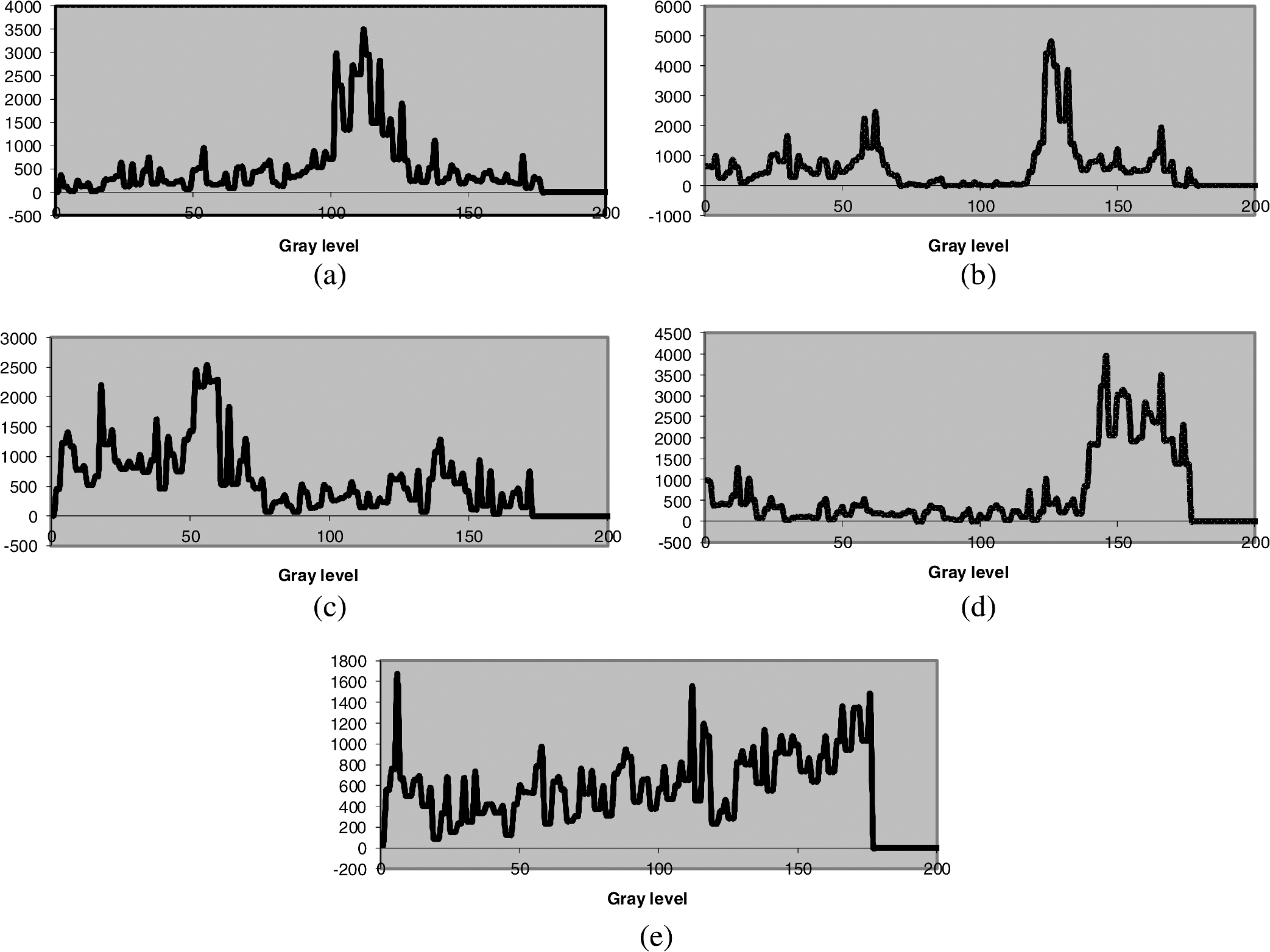
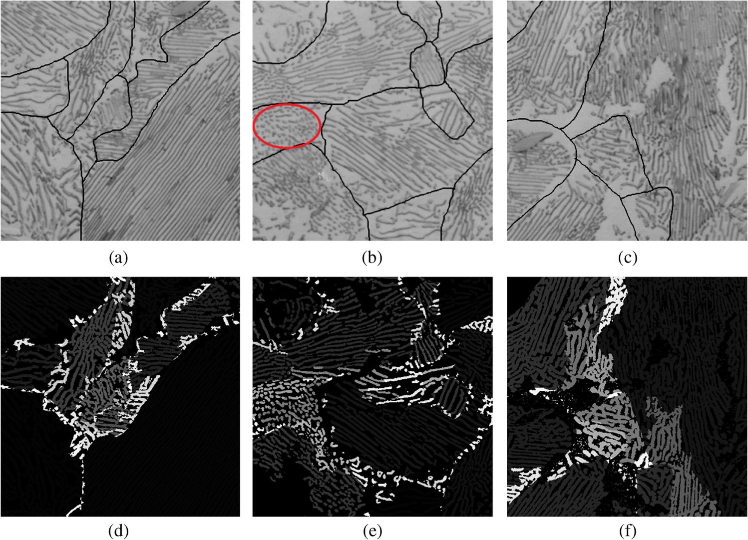
Fig. 4

Fingerprint segmentation based on a composition of connections. (a) Original image $X$ , (b) and (c) connected components according to $κ_{y}^{45,20,135, 10}$ and $κ_{y}^{60,20,150, 10}$ , (d) largest connected component $A_{1}$ , (e) residue $X ∖ A_{1}$ , (f) five connected components, (g) geodesic mask, (h) and (i) segmented image.

Depending on the images (fingerprint or pearlite phase images), the method requires a careful examination of the images to establish the largest size of the directional openings $λ_{1}$ and the amount $Δ λ_{1}$ to decrease the scale $λ_{1}$ .Conversely, the $λ_{2}$ parameter is very robust, and the size $λ_{2} = 5$ works correctly for all images. Figure 4 illustrates the performance of the algorithm. The image in Fig. 4(f) shows five connected components computed by this procedure. This is the partial partition $P p (X)$ . The idea of computing the final partition comes from the work of Ronse,³² and it consists of building the influence zones of the connected components in Fig. 4(f) inside the image in Fig. 4(g). This last image was computed from the set $X$ by applying a morphological closing. The influence zones are illustrated in Fig. 4(h). Figure 4(i) shows the final partition. The main problem of this method is the establishment of paramenters $λ_{1}$ and $Δ λ_{1}$ , which it will be described in Sec. 5. In the next section, a method not requiring these parameters is introduced.

4. Histogram-Based Segmentation Using the Orientation Partition Function

In this section, an approach to decrease the complexity of the segmentation problem is introduced. The flow chart in Fig. 5 illustrates the different steps to carry out a segmentation. It consists of codifying the size and orientation of the structures by means of two functions: viscosity $(V f_{X})$ and orientation $(O m_{X})$ . Then, a method to establish relationships between maxima of the viscosity function is proposed. This information is codified in a gray-level image called OPF. Subsequently, a systematic merging process is performed on this image to obtain the final segmentation based on the histogram of the OPF. Finally, in the last step, small regions are removed.

Fig. 5

Flow chart of the segmentation process.

4.1.

Size and Orientation Codification Based on Viscous Connectivity

A method to characterize the orientation field was proposed by Soille and Talbot.¹ The directional morphological openings and closings are used to filter bright and dark structures, respectively. Among the different functions proposed by the authors for codifying structures, the following functions were used to extract the orientation information of the images.

Eq. (8)

{Dir}_{λ}^{+} = {α_{i} : γ_{α_{i}, λ} \geq γ_{α_{j}, λ}, \forall α_{j} \neq α_{i}} {Dir}_{λ}^{-} = {α_{i} : φ_{α_{i}, λ} \leq φ_{α_{j}, λ}, \forall α_{j} \neq α_{i}} .

Particularly in fingerprints, the function ${Dir}_{λ}^{+}$ is used to extract the orientation of bright ridges, whereas ${Dir}_{λ}^{-}$ enables the extraction of dark ridges. This approach is general in different aspects: it can be applied to gray-level and binary images, and to all types of images containing directional structures. Here, we are strictly interested in segmenting images that can be considered binary images, as those in Fig. 1. We are looking for an approach where the scale and orientation information of the structures of the image are easily accessible to determine its connected components. First, let us define the directional structures of an image by assigning a viscosity to each pixel in the image. Each point of the structure is described by two quantities: the angle to the horizontal axis and a weight. Orientations have a periodicity of 180 deg in comparison to vectors, which have a periodicity of 360 deg. On the other hand, the weight will be given by the largest viscosity element, i.e., the longest line segment completely included in the structures. Two functions that codify the directional structures, by size and orientation, are introduced below. First, let us define a new function that codifies size information.

Definition 3.

The viscosity function $V f_{X} (x)$ is a transformation that associates the largest viscosity $λ$ with each pixel $x$ of a set $X$ .

Eq. (9)

V f_{X} (x) = V {λ | x \in \underset{α \in [0,180]}{V} {ε_{α, λ} (X)}} .

A way to compute this function is as follows. Let $X$ be a given set; one begins with a small structuring element by taking into account all orientations to compute the set $\underset{α \in [0,180]}{V} {ε_{α, λ} (X)}$ . This means that all the points of the image selected are those not removed by at least one of the directional erosions. Next, $V f_{X}$ is increased by one at all points $x$ belonging to the set $\underset{α \in [0,180]}{V} {ε_{α, λ} (X)}$ ; this procedure is continued by increasing the size of the structuring element until the structure (the image) is completely removed. This means the procedure is carried on until a $λ_{\max}$ value is obtained such that $V_{α \in [0,180]} {ε_{α, λ_{\max}} (X)} \neq \emptyset$ and $V_{α \in [0,180]} {ε_{α, λ_{\max} + 1} (X)} = \emptyset$ . As expressed before, the gray levels of the function $V f_{X}$ are the sizes of the longest lines that can be included in the structure. For the structures that can be considered as composed by a set of lines [Figs. 1(a) and (b)], the maxima of the function $V f_{X}$ play a main role since they codify the longest lines that take into account the whole context of the image. In this manner, the position of the largest structuring elements that are completely included in the structure is obtained by means of the maxima of $V f_{X}$ . However, the angles of these structuring elements (line segments) are not accessible from the image $V f_{X}$ . Therefore, a second function associated with the viscosity function needs to be introduced.

Definition 4.

The orientation function $O m_{X} (x)$ is a transformation that associates the angle of the viscosity in $V f_{X} (x)$ with each pixel $x$ of a set $X$ .

The directions of the line segments are stocked in a second image $O m_{X}$ called orientation function, when the viscosity function is computed. Figure 6 shows an interesting example where the maxima play a fundamental role to characterize the directional information. Figures 6(b) and 6(c) illustrate the viscosity and orientation functions, respectively, computed from the image in Fig. 6(a), whereas the image in Fig. 6(d) displays the original image and the maxima (in white) of the viscosity function. Particularly, observe that there exists only one maximum for each component. The viscosity and orientation functions can be used for extracting the line segments characterizing the structure. To illustrate the information contained in these images, a line segment of size $V f_{X} (x)$ was placed at each maximum point “ $x$ ,” with an angle given by the image $O m_{X} (x)$ . This reconstruction can be observed in Fig. 6(e). It seems that maxima are good features to describe directional structures. Let us illustrate this reconstruction with a real example (pearlitic phase micrograph) that is shown in Fig. 7. The images in Figs. 7(b) and 7(c) illustrate the image of the viscosity function $V f_{X}$ and the image containing the orientation $O m_{X}$ , respectively, computed from the binary image in Fig. 7(a). Finally, the image in Fig. 7(d) has been reconstructed using the respective viscosity and orientation functions. Only the maxima of the viscosity function were used in the reconstruction. Therefore, we can observe that both features, the maxima of the viscosity function and the orientation function, play a main role to extract directional structures. The maxima of $V f_{X}$ and the orientation image will be used to propose a method for segmenting the images.

Fig. 6

Viscosity and orientation functions. (a) Original image. (b) Viscosity function. (c) Orientation function. (d) Maxima of the viscosity function (in white) and original image. (e) Reconstructed objects.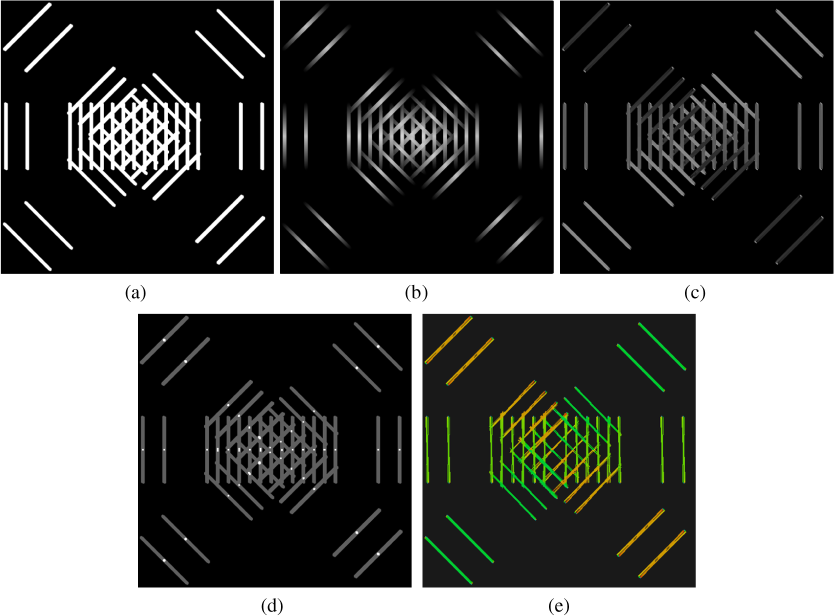

Fig. 7

Orientation partition function. (a) Original image. (b) and (c) Viscosity and orientation functions, respectively. (d) Reconstructed image. (e) and (f) Maxima of the viscosity function and its image partition computed by the watershed transformation. (g) Catchment basins of the partition weighted by the orientation partition function (OPF). (h) Orientation representation of image using the OPF.

4.2.

Orientation Partition Function

Since the maxima of the viscosity function and their orientations codified in the orientation function play a main role to reconstruct the original image, we propose method to establish the relationships among the maxima of the viscosity function. The main idea in this approach consists of building an image that codifies the neighborhood relations between the maxima and their orientations. A transformation that takes into account these relationships among maxima is the watershed, by working with the inverse image of $V f_{X}$ . Therefore, this transformation will be used to find basic relations between the connected components (characterized by maxima). However, instead of using the watershed lines, the catchment basins associated with the watershed will be used. In fact, the catchment basins related to the maxima can be computed by means of geodesic dilations. Figure 7(e) shows the maxima of the image $V f_{X}$ in Fig. 7(b), whereas Fig. 7(f) illustrates the watershed image computed from the inverse image of $V f_{X}$ . Figure 7(g) shows the catchment basins weighted by the values of the angles of the $O m_{X}$ image in Fig. 7(c) at the position of the regional maxima. This new function in Fig. 7(g) is the OPF, whereas the image in Fig. 7(h) is the representation of the orientation of the image in Fig. 7(a) using the OPF. By analyzing a region of the image in Fig. 7(g), one can identify the neighboring regions presenting similar orientations. These regions may belong to the same connected component. To take into account these neighborhood relationships, the histogram of the OPF will be used to carry out the merging process.

4.3.

Histogram-Based Segmentation

In this section, we discuss an approach for segmenting directional structures based on the histogram of the OPF. It is well-known that this approach can yield very good results when the objects have distinct ranges of intensity. This is not strictly the case for directional structures; however, in the case of fingerprints, the following hypothesis can be posed: two neighboring regions in the image have neighboring values in the histogram of orientations. Hence, the spatial analysis is practically equivalent to the gray-level analysis in the histogram. In the case of pearlite phase images, one assumes that the intensities have distinct ranges in the OPF. This hypothesis is supported by the fact that the grain structure displays a morphology in the form of parallel lines, and when forming another grain, these change direction. In this case, the histogram segmentation approach can also be used for segmenting the images.

Thus, after computing the histogram $H$ of the OPF associated with the original image, the histogram is clustered independently by splitting it into several sections corresponding to representative classes of pixels in the image. Therefore, the segmentation problem is reduced to finding the threshold values that dissect the histograms in a finite number of clusterings. Adjacent sections of the histogram will be merged according to the following strategy. A one-dimensional (1-D) adjacency graph of the histogram sections is built, and the two adjacent sections showing the smallest value of a given criterion in the histogram are identified and merged. The procedure of merging adjacent regions is carried out until a number of predefined classes is achieved. This solution that resembles the supervised approach proposed by Lezoray⁴³ enables a reduction in the number of regions of the OPF in an optimal manner. Several criteria for merging adjacent sections were studied. However, the best results were found by using the gray-level variance of the regions represented by two adjacent sections of the histogram. Let $S_{i}$ be the sections of histogram $H$ , with $i \in {0, 1, 2, \dots, 179}$ . The variance value is given by

Eq. (10)

σ (S_{i - 1}, S_{i}) = \sqrt{\frac{\sum_{k \in l (S_{i - 1})}^{u (S_{i})} H {(k)}^{2} {(k - μ)}^{2}}{\sum_{k \in l (S_{i - 1})}^{u (S_{i})} H (k)}},

where the mean value

μ

is

Eq. (11)

μ (S_{i - 1}, S_{i}) = \frac{\sum_{k \in l (S_{i - 1})}^{u (S_{i})} H (k) * k}{\sum_{k \in l (S_{i - 1})}^{u (S_{i})} H (k)} .

H (k)

is the number of pixels of gray level

k

and

l (S_{i})

[resp.

u (S_{i})

] is the lowest (resp. highest) gray level in section

S_{i}

. The adjacency graph is updated each time two sections are merged and the algorithm is iterated until the number of sections in the histogram is

N_{s}

. Figure 8 illustrates some segmented images for different

N_{s}

values. The output images in Figs. 8(b) to 8(f) were computed from the original image in Fig. 8(a) using

N_{s} = 8, 6, 5, 4, 3

, respectively. The segmented images form a hierarchy of partitions depending on the

N_{s}

parameter. Thus, let

P_{N_{s}} (f)

be the segmented image of

f

. With regard to partitions, one has that for any

i

and

j

with

j < i

,; this implies that

P_{i} (f) \subset P_{j} (f)

. It is clear that the number of regions of the segmented images does not correspond to the number of selected clusters

N_{s}

as shown in Fig. 8. However, despite this lack of correspondence, these images are practically segmented in the main regions. For example, to compute the image in Fig. 8(f), the selected number of sections of the histogram was

N_{s} = 3

, but the segmented image has the four largest regions that are representative of the directional structures of the image in Fig. 8(a).

Fig. 8

Histogram-based segmentation. (a) Original image. (b) to (f) Segmented images using variance criteria $N_{s} = 8$ , 6, 5, 4, 3, respectively. (g) The four largest regions of image (f). (h) Mask image. (i) Influence zones of (g) inside (h).

4.4.

Removal of Small Regions

Even when the output images computed by the histogram-based segmentation contain large representative regions, the method also generates small classes as those signaled by an arrow in Fig. 8(f). Small classes turn out to be inherent in segmenting techniques. To remove these regions, another approach, such as the use of the regions adjacency graph (RAG) structure, could be used for obtaining the final segmentation. By merging neighboring regions with close values in the gray level (orientation criterion) using the RAG, the order between partitions is preserved. Nevertheless, two main problems arise when removing small regions with the RAG structure: the complexity of the method and the fact that small regions have no correlation with their neighboring ones. For instance, the small regions signaled by an arrow in Fig. 8(f) have a gray level (orientation) that is not close to the gray level of the neighboring region, which means that a large criterion value is required to merge these regions. A large value of the criterion carries the risk of merging representative regions. Thus, we prefer to use a recent and formal approach proposed by Serra,⁴⁴ which also preserves an order. Serra establishes what he calls grain building ordering. Consider two partitions $P_{A}$ and $P_{B}$ . Then,

P_{A} ⪯ P_{B} when each class of P_{B} contains at least one class of P_{A} .

It does not preserve inclusion since some connected classes of the smaller partition, $P_{A}$ , may lie partly or even completely outside of $P_{B}$ . Figure 8 illustrates this concept. The image in Fig. 8(g) (partition $P_{B}$ ) has been computed by removing the small regions of the image in Fig. 8(f) (partition $P_{A}$ ). Only the four largest regions remain intact. Now, to compute the output image in Fig. 8(i), the influence zones of the connected components in Fig. 8(g) are built inside the mask in Fig. 8(h). This new partition, say $P_{C}$ , is greater than partition $P_{A}$ , i.e., the order is preserved ( $P_{A} ⪯ P_{C}$ ). This is a most interesting method for removing small regions given its simplicity and perfomance, which will be illustrated in the next section.

5. Results and Discussion

5.1.

Image Segmentation Based on the Connectivities Generated by Openings and Dilations

The first algorithm described in Sec. 3 has been tested on several images with good results. Here, we illustrate other examples and comment on some drawbacks of the approach. Figure 9 shows two examples of segmented images. Figure 9(b) shows the connected components computed from Fig. 9(a) using this procedure, whereas Fig. 9(d) displays the influence zones inside the mask in Fig. 9(c), and Fig. 9(e) shows the segmented image. Another example is illustrated in Fig. 9(f). Figure 9(g) shows seven connected components computed by the mentioned algorithm, whereas Figs. 9(h) and 9(i) display the segmented image. In this last example, the influence zones of the connected components in Fig. 9(g) are built using the whole image as a mask. However, there are some drawbacks in this method. One problem is the need for determining the values of parameters $λ_{1}$ and $Δ λ_{1}$ , and a second one is the large computation time. With regard to the former, it requires to carry out some experiments to select the largest scale $λ_{1}$ and the decrease $Δ λ_{1}$ . This can be avoided by computing all the scales as in the viscosity function; nevertheless, it risks to increase considerably the computation time.

Fig. 9

Examples of segmentation based on a composition of connections. (a) Original image $X$ . (b) Connected components. (c) Mask image. (d) Influence zones of connected components in (b) inside the mask image in (c). (e) Segmented image. (f) Original image. (g) Connected components. (h) and (i) Segmented image.

Now, concerning the latter problem, even computing few connected components, the method is slow when compared with the other one that uses the OPF and the histogram-based segmentation. Let us illustrate the number of operations requiered by this algorithm. We express the computational time in terms of basic erosions and dilations (size 1), and one considers that the contribution of the basic erosion and dilation is the same. Principally, two steps of the algorithm involve a considerable amount of computational time: the use of openings and dilations to compute the connected components at each orientation, and the selection of the largest connected component. To determine the first connected component, one needs to apply $2 λ_{1}$ erosions and dilations (directional openings of size $λ_{1}$ ), followed by $λ_{2}$ dilations. These transformations are applied at each point of the image and for all direction $α$ ; this means $(180 / Δ α) \cdot (2 λ_{1} + λ_{2})$ basic operations for each point of the image, where $Δ α$ is the angle step ( $Δ α = 5$ for the examples in Fig. 9). Moreover, this is the number of operations for each connected component; then $NC (180 / Δ α) (2 λ_{1} + λ_{2})$ operations are necessary to obtain the segmented image. Regarding the second step—the selection of the largest connected components—it also requires $NC (180 / Δ α) (2 λ_{1} + λ_{2})$ scannings of the image. Therefore, the number of scannings required to compute the segmented image makes the algorithm very slow.

5.2.

Some Comments About the Codification of Size and Orientation

In Sec. 4, when the viscosity and orientation functions were introduced, we claimed that the pair of data, maxima of the viscosity function and their orientations, contains the main information of the original structures. This hypothesis was later used to build the OPF to segment the images. Before establishing this hypothesis, several experiments were carried out with a set of images. Figures 10(f) to 10(j) illustrate some examples of reconstructed images. The reconstruction percentage is $\sim 63 %$ , which seems small. However, by comparing the images in Figs. 10(f) to 10(j) and those of Figs. 10(a) to 10(e), we appreciate that the reconstructed images are representative of the original images since they contain the main shapes. The remaining information is redundant. Then, the maxima of the viscosity function play a crucial role in the characterization of directional structures. Moreover, the orientation function faithfully represents the shape of the structures. Let us illustrate this assertion with examples. Figures 11(b) and 11(c) show the viscosity function and its associated orientation function of the original image in Fig. 11(a). In addition, a color representation of the orientation function is also shown in Fig. 11(d). The gray-level orientation image enables the introduction of a connectivity criterion. Figures 11(e) and 11(f) illustrate the connectivity introduced by the orientation of the structures. The image in Fig. 11(e) was computed from the image in Fig. 11(c) using a threshold between 160 and 172 deg (gray levels in the image). Then, by using the arc-wise connectivity, the number of connected components between these angles can be determined. Similarly, for the image in Fig. 11(f), the number of connected components with an orientation lying between 92 and 152 deg can also be computed.

Fig. 10

Examples of reconstructed images using the máxima of the viscosity function. (a) to (e) Original images. (f) to (j) Reconstructed images.

Fig. 11

Extraction of connected components using the orientation function. (a) Binary image. (b) Viscosity function. (c) Orientation function. (d) Color representation of (c). (e) Threshold between 160 and 178 gray levels computed from the image in (c). (f) Threshold between 92 and 152 gray levels computed from the image in (c).

Now, Fig. 12(a) illustrates a real example having similar directional structures as those of the image in Fig. 11(a). In Fig. 12(b), the orientation function in color representation is shown. To extract directional structures, a threshold in a given interval is applied to this last image. For instance, the image in Fig. 12(c) was computed using a threshold between 100 and 180 deg (gray levels in the orientation function). A main structure and some small ones are observed in this image. In order to extract the principal structure, a directional dilation at 45 deg (more or less perpendicular to the main structure) is applied to the image in Fig. 12(c) to compute the image in Fig. 12(d). Next, the largest connected component is extracted as shown in Fig. 12(e). A similar procedure is carried out for computing other directional structures, as displayed in Fig. 12(f). Finally, one builds the influence zones of the regions in Fig. 12(f) inside the image in Fig. 12(g). Figures 12(h) and 12(i) show the segmented image. Even if this algorithm is very fast, particularly when the method proposed below in Sec. 5.5 to compute the viscosity and orientation functions is applied, the main problem lies in the fact that it is not easy to compute an optimal segmentation.

Fig. 12

Example of segmentation using the orientation function. (a) Binary image. (b) Orientation function. (c) Threshold between 100 and 180 gray levels computed from the image in (b). (d) Directional dilation at 45 deg. (e) Largest connected component. (f) Four connected components. (g) Mask image. (h) and (i) Segmented image.

5.3.

Some Comments About the Histogram-Based Segmentation

In the proposed algorithm for the histogram-based segmentation in Sec. 4, all the sections of the histogram were used for segmenting the images. However, in a first solution, one may suppose that the representative sections (clusters) of the histogram are located around the regional maxima. Let us illustrate some problems using this assertion. Figures 13(a) to 13(e) show the OPFs of the original images in Figs. 10(a) to 10(e), whereas in Figs. 14(a) to 14(e), the histograms of the OPFs are illustrated. Several comments about the behavior of the histograms can be made. First, observe that a main representative section in the histogram, linked to a principal directional structure, is always present and this behavior is reflected in the histogram by a wide section, such as those of Figs. 14(a) and 14(d). Even in the case of the histogram shown in Fig. 14(e), corresponding to the OPF image in Fig. 10(e), this main structure is present and can be detected. Nevertheless, small representative directional regions are also included and can be also detected by a clustering process carried out in the histogram.

Fig. 13

Examples of OPFs. (a) to (e) OPFs of the images in Figs. 10(a) to 10(e), respectively.

Fig. 14

Histograms of OPFs. (a) to (e) Gray-level histograms of Figs. 13(a) to 13(e), respectively.

Now, as expressed above, a first solution for dissecting the histogram can be achieved by computing a 1-D watershed of the complement ( $H^{c}$ ). Then, maxima of $H$ (minima of $H^{c}$ ) are supposed to mark the main regions of the images. Nevertheless, one observes that maxima are numerous in the histograms of Fig. 14; this may cause an oversegmentation problem. Instead of using the minima of $H^{c}$ , one can use the so-called h-minima as seeds for the 1-D watershed. This avoids oversegmentation. This idea of segmenting images comes from the work of Lezoray.⁴³ However, the major drawback of this approach for selecting the main regions of the structure does not always yield good results, that is, the maxima of the histogram are not strictly representative of the principal structures. Moreover, when an angle step $Δ α$ different from 1 deg is used for computing the OPF as illustrated in Fig. 15, all the values in the histogram, multiple of $Δ α$ are maxima. This is the reason why in the algorithm proposed in Sec. 4 we take all the possible regions in the histogram with the same gray level for segmenting the images. This means, 180 sections for $Δ α = 1$ , or 90 sections for $Δ α = 2$ , and so on.

Fig. 15

Examples of histograms of OPFs. (a) and (b) OPF using a five-degree step and its corresponding histogram. (c) and (d) OPF using a 10-degree step and its corresponding histogram.

To illustrate the performance of the histogram-based segmentation approach using the OPF, several examples are displayed in Figs. 16 and 17. First, we show the segmentation process in the fingerprint case. The images in Figs. 16(e) to 16(h) were computed from those in Figs. 16(a) to 16(d) using the histogram-based segmentation. All segmented images present small regions. For removing these regions, the method described in Sec. 4.4, based on the concept of grain building ordering, was applied to the images in Figs. 16(e) to 16(h). The images in Figs. 16(i) to 16(l) illustrate the final segmentations. In addition, Fig. 17 shows the examples of pearlite phase images. They have been segmented using the histogram-based segmentation approach followed by the algorithm for removing small regions. Figures 17(b) and 17(c) illustrate the segmented images computed from the image in Fig. 17(a), whereas in Figs. 17(d) and 17(e) two grains are shown. Finally, Figs. 17(f) and 17(h) show two last examples of pearlite phase images, and in Figs. 17(g) and 17(i) their respective segmented images in color representation are shown as well.

Fig. 16

Examples of the histogram-based segmentation. (a) to (d) Original images. (e) to (h) Segmented images using variance criteria $N_{s} = 4$ . (i) to (l) Segmented images corresponding to those of (e) to (h) without small regions.

Fig. 17

Pearlitic phase image segmentation. (a) Original image. (b) Segmented image using variance criterion $N_{s} = 4$ . (c) Color representation. (d) and (e) Two connected components. (f) and (g) Original and segmented images using variance criterion $N_{s} = 4$ . (h) and (i) Original and segmented images using variance criterion $N_{s} = 4$ .

Now, let us make some comments concerning the computation time of the method. Four steps are required to obtain the segmented image as shown in Fig. 5. Three of them are determined very fast: OPF determination, histogram-based segmentation, and small regions removal. The step that involves a considerable amount of operations is the computation of the viscosity and orientation functions. Unlike the method based on the composed connectivities (Sec. 3) that uses openings and dilations, this step requires only erosions. If these functions are computed using Eq. (9) directly, the method becomes very slow, $(180 / Δ α)$ erosions at each point of the image for every scale $λ$ . However, by using the algorithm described below in Sec. 5.5, the computation time is considerably reduced. The idea in the algorithm described below consists of determining the critical line segments at each point of the image, i.e., the longest line segments that can be placed inside the structure. Once the viscosity and orientation functions are calculated, they are used for the computation of the OPF, which needs only one scanning to obtain the catchment basins associated to the watershed. The existence of an efficient algorithm to compute the watershed is well-known. Regarding the histogram-based segmentation, the computation time is negligible since this step involves the calculation of Eqs. (10) and (11) on a vector of length 180. Finally, the removal of small regions is also a fast algorithm given that two procedures are only required: computation of the largest regions and the influence zones determination.

5.4.

Comparison of the Method with Manual Segmentation of Pearlitic Phase Images

To test the performance of the method based on the OPF and histogram-based segmentation, the segmented images from this algorithm were compared with manual segmentations carried out by a materials science specialist. To our knowledge, the work of Jeulin and Kurdy³ is the only article addressing the segmentation of pearlite phase images. Since in their work there is no comparison of their method, we decided to evaluate the performance with the ground truths provided by an expert. There are several works in the literature focused on testing segmented images with ground truths (see Refs. 45 46. to 47). Here, we will focus on the use of the index proposed by Martin et al.⁴⁵ Let $P (f)$ and $P_{M} (f)$ be the partition computed from image $f$ using the proposed method and the ground truth, respectively. Let $∖$ denote the set difference and $| A |$ the cardinality of set $A$ . If $P (f) (x)$ is a region (class or element of the partition) at point $x$ in the segmentation $P (f)$ , the local refinement error between the classes $P (f) (x)$ and $P_{M} (f) (x)$ is defined as

Eq. (12)

E [P (f) (x), P_{M} (f) (x)] = \frac{| P (f) (x) ∖ P_{M} (f) (x) |}{| P (f) (x) |} .

Note that this local error encodes a measure of refinement in one direction only. When $P (f) (x)$ is a refinement of $P_{M} (f) (x)$ the error is zero. Given this local refinement error at each direction for each pixel $x$ , a way to combine the values into an error measure for the entire image is the local consistency error. Let $N$ be the number of pixels of the image. Then

Eq. (13)

LCE (S_{1}, S_{2}) = \frac{1}{N} \sum_{i} \min {E [P (f) (x), P_{M} (f) (x)], E [P_{M} (f) (x), P (f) (x)]} .

Now, the images were manually segmented by the specialist as illustrated in Figs. 18(a) to 18(c). The error $\min {E [P (f) (x), P_{M} (f) (x)], E [P_{M} (f) (x), P (f) (x)]}$ was computed at each point of the image between the ground truth images and those segmented by the proposed method [Figs. 17(c), 17(g), and 17(i)]. The images in Figs. 18(d) to 18(f) illustrate this error. We observe that the error is greater for the border pixels [white color in Figs. 18(d) to 18(f)], whereas it is smaller (dark regions) for larger well-defined grains. See, for example, the image in Fig. 18(d). Another source of error is not well-defined grains. See, for example, the region (red ellipse) of the image in Fig. 18(b) and its corresponding error image in Fig. 18(e). In this region, the pearlite phase does not display a morphology in the form of parallel lines. Similarly, when one has small grains, neighboring of a larger one, it is not possible to carry out a proper segmentation as shown in Fig. 18(f). However, from a practical point of view, the pearlite phase images are, in general, segmented correctly. Finally, the mean error was computed on a set of images using Eq. (12), finding a value of 0.19.

Fig. 18

Comparison of the histogram-based segmentation method with manual segmentations. (a) to (c) Ground truth images. (d) to (f) Error $\min {E [P (f) (x), P_{M} (f) (x)], E [P_{M} (f) (x), P (f) (x)]}$ .

5.5.

Nonparametric Algorithm to Build the Viscosity and Orientation Functions

The number of operations needed for computing the viscosity and the orientation functions is considerable, making this a very expensive method in computation time. Moreover, the building of these functions seems to require a size parameter (the largest structuring element) and an angle step to compute them. Let us illustrate an algorithm to build these functions, which does not require any parameter and is not expensive in computation time. First, the size parameter (largest structuring element) can be fixed to the size of the image diagonal, that is, the size of the largest structure that can be included in the image. Let $S_{x}$ and $S_{y}$ be the dimensions of the images in the horizontal and vertical axes, respectively. For example, for a VGA $640 \times 480$ image, one has $L = \sqrt{S_{x}^{2} + S_{y}^{2}} = 800$ . Then the largest structuring element has a size of 400 since one uses symmetrical structuring elements. It is clear that few cases of images containing such structure characteristics can be found in real images. Next, to compute the line segments, the step in degrees must be fixed. In practice, a 5-deg step ( $Δ α$ ) is sufficient, but let us fix a smaller value (1 deg) to show the limiting case in computation time. Figures 19(a) to 19(c) show the line segments of size 200 for angle steps of 10, 5, and 1 deg, respectively. Next, 180 structuring elements of size L are computed and stocked in a structure data (list of lists). Since symmetrical structuring elements are used, only half of the straight lines are stocked and centered at the origin $(0, 0)$ . In fact, only the Freeman codes are stocked. Let ${L s_{i}}$ with $i \in {0, 1, 2, \dots, 179}$ be the lists containing the Freeman codes required to build half of the structuring elements, and let $L s_{j}$ be a given list. The structuring element is built using the list $L s_{j} = {c_{k}}$ with $c_{k} \in {0, 1, 2, 3, \dots, 7}$ and its symmetrical data $\overset{˘}{L} s_{j} = {{\overset{˘}{c}}_{k}}$ with ${\overset{˘}{c}}_{k} = (c_{k} + 4) \mod 8$ .

Fig. 19

Algorithm to build $V f_{X}$ and $O m_{X}$ images and some geometrical examples. (a) to (c) Line segments size 200, with step angles of 10, 5, and 1 deg, respectively. (d) and (e) Directional erosions. (f) and (g) Rectangular structures with their orientation functions. (h) and (i) Original structure and its orientation function.

To illustrate the algorithm, let us consider the example in Fig. 19(d), where an erosion by a line segment is applied to the structure in gray color. The structuring element is obtained from the list $L s_{j} = {0, 1, 0, 1, 0, 1, 0, 1, 0}$ (blue 0 and red 1) and $\overset{˘}{L} s_{j} = {4, 5, 4, 5, 4, 5, 4, 5, 4}$ (green 4 and yellow 5). Now, to calculate the erosion at point $(x, y)$ of an image $f$ marked by a white dot, one begins by computing the smallest value among the points $(x - 1, y)$ , $(x, y)$ , and $(x + 1, y)$ . Then, the erosion size 1 is given by the infimum (the intersection of sets) $ε_{1} (f) (x, y) = f (x - 1, y) Λ f (x, y) Λ f (x + 1, y)$ . Next, the erosion size 2 is obtained by using the following two points of the structuring element $(x - 2, y - 1)$ and $(x + 2, y + 1)$ and the erosion size 1 $ε_{1} (f) (x, y)$ . Hence, $ε_{2} (f) (x, y) = f (x - 2, y - 1) Λ ε_{1} (f) (x, y) Λ f (x + 2, y + 1)$ . The procedure continues until the last pair of points of the structuring element is taken into account. In this example, a longer structuring element is required to remove the point $(x, y)$ of the image. Nevertheless, in the example in Fig. 19(e), after applying the third erosion, the point is removed; i.e., $ε_{3} (f) (x, y) = f (x - 3, y - 2) Λ ε_{2} (f) (x, y) Λ f (x + 3, y + 3) = 0$ . Hence, the procedure is stopped. This process is applied to each point of the image. It is clear that the fact of using the infimum (AND operation in a computer) to compute the erosion and to stop the procedure when it is no longer required allows a faster calculation of the erosion of the image. Then, instead of calculating $V_{α \in [0,180]} {ε_{λ, α} (X)}$ , one computes at each point $x$ of the image, the longest structuring element that cannot remove this point. Subsequently, the length of this structuring element is used to affect the function $V f_{X}$ at point $x$ .

Now, in order to know approximately the time complexity order for computing the viscosity and orientation functions, let us consider the limit case of a structure composed of a line segment at direction $α = 0$ , 1 pixel thick and $2 * n + 1$ pixels in length, with $n ≫ 1$ . To compute the critical elements of the supremum of erosions at the center $x$ of the line segment, $n + 1$ directional erosions are required at direction $α$ , plus (approximately) $m$ erosions for the other angles. The value $m ≪ n$ , depends on the angle of the directional erosion. It is 1 for an angle perpendicular to $α$ and is a maximum $m$ for an angle close to $α$ , according to a given angle step $Δ α$ . For example, for $Δ α = 5$ , one has more or less $m = 5$ . For the other points of the line segment, the number of operations depend on the point position, and their values are between 1 and $n$ at direction $α$ and $m$ erosions for the other angles. Hence, the number of directional erosions required to test all points is ${(n + 1)}^{2} + (180 / Δ α) * m * n$ . Let us illustrate an example. For a line segment of length $n = 99$ and $Δ α = 5$ , 10,000 erosions are required at the direction $α [term {(n + 1)}^{2}]$ , whereas for other angles (term $m * n$ ) between 100 and 500 erosions. Now, for a line segment of thickness 2 pixels, one has approximately $2 * [{(n + 1)}^{2} + (180 / Δ α) * m * n]$ . By increasing the thickness of the line segment, the determination of the time computation order becomes more complex. Then, for thin ( $k$ pixels) and long segments, a good value for the order is $k * [{(n + 1)}^{2} + (180 / Δ α) * m * n]$ .

Finally, let us show the computation time of the present approach. For instance, in the example of the pearlitic phase image of size $512 \times 512 pixels$ , 5 s are required to compute the viscosity and orientation images using a 1-deg angle step, whereas when working with a 5-deg step in the interval [0,180], only 1 s is required. For the fingerprint image ( $300 \times 300 pixels$ ), $< 2 s$ are required using a 1-deg angle step. The computer used for these experiments was a laptop with 1.59 GHz processor and 256 MB RAM.

5.6.

Limits of the Approach

Let us take some geometrical examples to illustrate certain limitations of the approach proposed above using the OPF to extract the directional characteristics. The first example is the case of a rectangle of length $l$ and width $h$ shown in Figs. 19(f) and 19(g). The longest line segments that can be placed inside the rectangle are the diagonal lines of length ${[l^{2} + h^{2}]}^{1 / 2}$ , and their angle is given by $α = \tan^{- 1} (h / l)$ . It is clear that the larger $l$ is, the smaller $h$ is, and the closer $α$ is to 0 deg ( $l \to \infty$ ; or $h \to 0, \Rightarrow α \to 0$ ). Consider an example where the rectangle has $l = 100$ pixels. Then, for $h = 20$ , $α = 11.5 \deg$ ; for $h = 10$ , $α = 5.7 \deg$ ; and for $h = 5$ , $α = 2.8 \deg$ . Another source of error is the rectangle extremes since, at the limits, the angle of the longest line (in this example) has an angle value of 90 deg. Moreover, the points remaining in the line that cuts the rectangle along the horizontal at $h / 2$ through its center can vary between $α = \tan^{- 1} (h / l)$ and 90 deg. Figures 19(f) and 19(g) show two examples in color representation. This drawback can be avoided by applying the supremum of directional openings; however, the computation time to determine the longest lines included in the structure will increase considerably. To illustrate this, let us remember the traditional geometrical interpretations of the erosion and the opening. In the erosion case, one selects the center of the structuring element that is completely included in the structure, whereas in the opening case, all the points hitting the structuring element are chosen. This means that when an opening is applied, the points in the image are analyzed several times, and it is not possible to apply the algorithm proposed above.

Now, let us analyze another geometrical example given by a shape formed by two concentric circles of different radii (annulus or ring of width $h$ ) as illustrated in Fig. 19(h). In the case of a disk, the maximum symmetrical distance lies in the middle point of the segment joining any two points of the circle (chord); the longest chord goes through the center of the disk (diameter of the disk). In the case of a ring, the longest line segment is the tangent to the inner circle, and the smallest line is zero, a point on the outer circle. Between these two extremes, different chords exist, all at the same angle. Then, when working with structures with a given curvature, the error in the direction is smaller than in the case of a straight line (or without error when the region takes a shape resembling a ring) as illustrated in Fig. 19(i). However, the maxima of the viscosity function will remain close to the contour (inner contour) of the structure. The limits of the approach shown in this section are attenuated when the image is composed of thin structures as those of the pearlitic phase micrograph or when the structures have curvatures as in fingerprint images.

6. Conclusion and Future Works

This paper shows the possibilities of applying the connectivity class notion to segment images containing directional structures. Initially, the composition of connections generated by the openings and dilations was investigated. This composition of connectivities is used to describe a class of hierarchical data structures, which allows the classification of the various orientations at different scales. The approach enables the correct segmentation of images containing directional structures; however, its computation time is large. Subsequently, a second local approach was considered. This approach involves a local analysis using the concepts of viscosity and orientation functions proposed in this paper. The maxima of the viscosity function were used for computing the loci of maximal structuring elements, and the orientation function to obtain the angles of the line segments. These pairs of local parameters yield a good description of the image by means of line segments. Subsequently, an OPF of the image was computed by means of the catchment basins associated with the watershed transform weighted by the orientation function. This method allows the segmentation of the image based on a supervised approach using the clustering of the OPF histogram. The results based on the algorithms presented in this paper show the good performance of the approach. Future work will consist of searching for segmenting images in the gray-level case, and we will focus on a new lattice approach for morphological image segmentation recently proposed by Serra.⁴⁸

Acknowledgments

We would like to thank the anonymous reviewers for their valuable comments and precisions. C. A. Paredes-Orta thanks the government agency CONACyT for the financial support. Also, the authors thank the material science specialists Julieta Torres-Gonzalez and Federico Castañeda for their help in the analysis of the pearlite phase segmented images. I. R. Terol-Villalobos would like to thank Diego Rodrigo and Darío T.G. for their great encouragement. This work was funded by the government agency CONACyT (133697), Mexico.

References

1.

P. SoilleH. Talbot, “Directional morphological filtering,” IEEE Trans. Pattern Anal. Mach. Intell., 23 (11), 1313 –1329 (2001). http://dx.doi.org/10.1109/34.969120 ITPIDJ 0162-8828 Google Scholar

2.

P. SoilleE. J. BreenR. Jones, “Recursive implementation of erosions and dilations along discrete lines at arbitrary angles,” IEEE Trans. Pattern Anal. Mach. Intell., 18 (5), 562 –567 (1996). http://dx.doi.org/10.1109/34.494646 ITPIDJ 0162-8828 Google Scholar

3.

D. JeulinM. Kurdy, “Directional mathematical morphology for oriented image restoration and segmentation,” Acta Stereologica, 11 (11), 545 –550 (1992). ASTLDL 0351-580X Google Scholar

4.

A. Tuzikovet al., “Extraction of grid patterns on stamped metal sheets using mathematical morphology,” in Proc. of the Eleventh Int. Conf. on Pattern Recognition, 425 –428 (1992). Google Scholar

5.

M. A. OliveiraN. J. Leite, “A multiscale directional operator and morphological tools for reconnecting broken ridges in fingerprint images,” Pattern Recognit., 41 (1), 367 –377 (2008). http://dx.doi.org/10.1016/j.patcog.2007.05.019 PTNRA8 0031-3203 Google Scholar

6.

I. R. Terol-VillalobosL. A. Morales-HernándezG. Herrera-Ruiz, “Directional structures detection based on morphological line-segment and orientation functions,” Lec. Notes Comput. Sci., 4992 458 –469 (2008). http://dx.doi.org/10.1007/978-3-540-79126-3 LNCSD9 0302-9743 Google Scholar

7.

L. A. Morales-HernándezI. R. Terol-VillalobosF. Manriquez-Guerrero, “Two approaches for orientation segmentation based on directional morphology,” in Proc. of the Eighth International Symp. of Mathematical Morphology and Its Applications to Image and Signal Processing, 325 –336 (2007). Google Scholar

8.

C. H. Parket al., “Singular point detection by shape analysis of directional fields in fingerprints,” Pattern Recognit., 39 (5), 839 –855 (2006). http://dx.doi.org/10.1016/j.patcog.2005.10.021 PTNRA8 0031-3203 Google Scholar

9.

J. LiW. Y. YauH. Wang, “Constrained nonlinear models of fingerprint orientations with prediction,” Pattern Recognit., 39 (1), 102 –114 (2006). http://dx.doi.org/10.1016/j.patcog.2005.08.010 PTNRA8 0031-3203 Google Scholar

10.

X. Chens, “PDE-based regularization of orientation field for low-quality fingerprint image,” in Proc. of the Eleventh IEEE Int. Conf. on Signal Processing, 1006 –1011 (2012). Google Scholar

11.

B. M. Popovicet al., “Different methods for fingerprint image orientation,” in Proc. of the 20th Telecommunications Forum, 662 –665 (2012). Google Scholar

12.

S. BharkadM. Kokare, “Fingerprint identification—ideas, influences, and trends of new age,” Pattern Recognition, Machine Intelligence and Biometrics, 411 –446 Springer, Berlin, Heidelberg (2011). Google Scholar

13.

H. HasanS. Abdul-Kareem, “Fingerprint image enhancement and recognition algorithms: a survey,” Neural Comput. Appl., 23 (6), 1605 –1610 (2013). http://dx.doi.org/10.1007/s00521-012-1113-0 0941-0643 Google Scholar

14.

J. K. LeeT. S. NewmanG. A. Gary, “Oriented connectivity-based method for segmenting solar loops,” Pattern Recognit., 39 (2), 246 –259 (2006). http://dx.doi.org/10.1016/j.patcog.2005.07.004 PTNRA8 0031-3203 Google Scholar

15.

C. Bahlmann, “Directional features in online handwriting recognition,” Pattern Recognit., 39 (1), 115 –125 (2006). http://dx.doi.org/10.1016/j.patcog.2005.05.012 PTNRA8 0031-3203 Google Scholar

16.

M. KassA. Witkin, “Analyzing oriented pattern,” Comput. Vis., Graph., Image Process., 37 (3), 362 –385 (1987). http://dx.doi.org/10.1016/0734-189X(87)90043-0 CVGPDB 0734-189X Google Scholar

17.

K. SandbergM. Brega, “Segmentation of thin structures in electron micrographs using orientation fields,” J. Struct. Biol., 157 (2), 403 –415 (2007). http://dx.doi.org/10.1016/j.jsb.2006.09.007 JSBIEM 1047-8477 Google Scholar

18.

A. M. BazenS. H. Gerez, “Systematic methods for the computation of the directional fields and singular points of fingerprints,” IEEE Trans. Pattern Anal. Mach. Intell., 24 (7), 905 –919 (2002). http://dx.doi.org/10.1109/TPAMI.2002.1017618 ITPIDJ 0162-8828 Google Scholar

19.

P. T. H. Trucet al., “Vessel enhancement filter using directional filter bank,” Comput. Vis. Image Underst., 113 101 –112 (2009). http://dx.doi.org/10.1016/j.cviu.2008.07.009 CVIUF4 1077-3142 Google Scholar

20.

C. K. WangY. H. Tseng, “DEM generation from airborne lidar data by an adaptive dual directional slope filter,” in Proc. of the Int. Society for Photogrammetry and Remote Sensing VII Symp., 628 –632 (2010). Google Scholar

21.

L. Zhonget al., “Handling noise in single image deblurring using directional filters,” in Proc. of the 26th IEEE Conf. on Computer Vision and Pattern Recognition, 612 –619 (2013). Google Scholar

22.

R. Rijiet al., “Fuzzy based directional weighted median filter for impulse noise detection and reduction,” Fuzzy Inf. Eng., 4 (4), 351 –369 (2012). http://dx.doi.org/10.1007/s12543-012-0120-2 1616-8658 Google Scholar

23.

E. Parra-DenisM. BilodeauD. Jeulin, “Multistep detection of oriented structure in complex textures,” (2013). Google Scholar

24.

S. KimJ. KoH. Chung, “Steel grade classification based on Gabor filters and K-means clustering,” in SERSC Int. Conf. on Circuits, Control, Communication, Electricity, Electronics, Energy, System, Signal and Simulation, 54 –57 (2013). Google Scholar

25.

J. Serra, Image Analysis and Mathematical Morphology, Vol. II, Theoretical Advances, Academic Press, New York (1988). Google Scholar

26.

H. J. A. M. Heijmans, Morphological Image Operators, Academic Press, New York (1994). Google Scholar

27.

P. Soille, Morphological Image Analysis: Principles and Applications, 2nd ed.Springer-Verlag, Heidelberg, Berlin (2003). Google Scholar

28.

U. Braga-NetoJ. Goutsias, “Connectivity on complete lattices: new results,” Comput. Vis. Image Underst., 85 (1), 23 –53 (2002). http://dx.doi.org/10.1006/cviu.2002.0961 CVIUF4 1077-3142 Google Scholar

29.

U. Braga-Neto, “Multiscale connected operators,” J. Math. Imaging Vis., 22 (2–3), 199 –216 (2005). http://dx.doi.org/10.1007/s10851-005-4890-6 JIMVEC 0924-9907 Google Scholar

30.

H. Heijmans, “Connected morphological operators for binary images,” Comput. Vis. Image Underst., 73 (1), 99 –120 (1999). http://dx.doi.org/10.1006/cviu.1998.0703 CVIUF4 1077-3142 Google Scholar

31.

Ch. Ronse, “Set-theoretical algebraic approaches to connectivity in continuous or digital spaces,” J. Math. Imaging Vis., 8 (1), 41 –58 (1998). http://dx.doi.org/10.1023/A:1008210216583 JIMVEC 0924-9907 Google Scholar

32.

Ch. Ronse, “Partial partitions, partial connections and connective segmentation,” J. Math. Imaging Vis., 32 (2), 97 –125 (2008). http://dx.doi.org/10.1007/s10851-008-0090-5 JIMVEC 0924-9907 Google Scholar

33.

C. RonseJ. Serra, “Geodesy and connectivity in lattices,” Fundadenta Informaticae, 46 (4), 349 –395 (2001). Google Scholar

34.

J. Serra, “Connectivity on complete lattices,” J. Math. Imaging Vis., 9 (3), 231 –251 (1998). http://dx.doi.org/10.1023/A:1008324520475 JIMVEC 0924-9907 Google Scholar

35.

J. Serra, “Viscous lattices,” J. Math. Imaging Vis., 22 (2–3), 254 –269 (2005). http://dx.doi.org/10.1007/s10851-005-4894-2 JIMVEC 0924-9907 Google Scholar

36.

C. S. TzafestasP. Maragos, “Shape connectivity: multiscale analysis and application to generalized granulometries,” J. Math. Imaging Vis., 17 (2), 109 –129 (2002). http://dx.doi.org/10.1023/A:1020629402912 JIMVEC 0924-9907 Google Scholar

37.

G. K. OuzounisM. H. F. Wilkinson, “Mask-based second-generation connectivity and attribute filters,” IEEE Trans. Pattern Anal. Mach. Intell., 29 (6), 990 –1004 (2007). http://dx.doi.org/10.1109/TPAMI.2007.1045 ITPIDJ 0162-8828 Google Scholar

38.

M. H. F. Wilkinson, “Attribute-space connectivity and connected filters,” Image Vis. Comput., 25 (4), 426 –435 (2007). http://dx.doi.org/10.1016/j.imavis.2006.04.015 IVCODK 0262-8856 Google Scholar

39.

I. Santillanet al., “Morphological connected filtering on viscous lattices,” J. Math. Imaging Vis., 36 (3), 254 –269 (2010). http://dx.doi.org/10.1007/s10851-009-0184-8 JIMVEC 0924-9907 Google Scholar

40.

J. Crespoet al., “A flat zone approach: a general low-level region merging segmentation method,” Signal Process., 62 (1), 37 –60 (1997). http://dx.doi.org/10.1016/S0165-1684(97)00114-X SPRODR 0165-1684 Google Scholar

41.

F. MeyerS. Beucher, “Morphological segmentation,” J. Vis. Commun. Image Represent., 1 (1), 21 –46 (1990). http://dx.doi.org/10.1016/1047-3203(90)90014-M JVCRE7 1047-3203 Google Scholar

42.

Ph. SalembierJ. Serra, “Morphological multiscale image segmentation,” Proc. SPIE, 1818 620 –631 (1992). http://dx.doi.org/10.1117/12.131477 PSISDG 0277-786X Google Scholar

43.

O. Lezoray, “Supervised automatic histogram clustering and watershed segmentation. application to microscopic medical color image,” Image Anal. Stereol., 22 (2), 113 –120 (2003). http://dx.doi.org/10.5566/ias.v22.p113-120 IASMCE 1580-3139 Google Scholar

44.

J. Serra, “Grain building ordering,” Lec. Notes Comput. Sci., 6671 37 –48 (2011). http://dx.doi.org/10.1007/978-3-642-21569-8 LNCSD9 0302-9743 Google Scholar

45.

D. Martinet al., “A database of human segmented natural images and its application to evaluating segmentation algorithms and measuring ecological statistics,” in Proc. of the Int. Conf. on Computer Vision, 416 –423 (2001). Google Scholar

46.

R. UnnikrishnanC. PantofaruM. Hebert, “Toward objective evaluation of image segmentation algorithms,” IEEE Trans. Pattern Anal. Mach. Intell., 29 (6), 929 –944 (2007). http://dx.doi.org/10.1109/TPAMI.2007.1046 ITPIDJ 0162-8828 Google Scholar

47.

J. Pont-TusetF. Marques, “Supervised assessment of segmentation hierarchies,” Lec. Notes Comput. Sci., 7575 814 –827 (2012). http://dx.doi.org/10.1007/978-3-642-33765-9 LNCSD9 0302-9743 Google Scholar

48.

J. Serra, “A lattice approach to image segmentation,” J. Math. Imaging Vis., 24 (1), 83 –130 (2006). http://dx.doi.org/10.1007/s10851-005-3616-0 JIMVEC 0924-9907 Google Scholar

Biography

Carlos A. Paredes-Orta received his BSc degree in computer engineering from the Instituto Tecnológico de Querétaro and his MSc degree in mechatronics from CIDESI, Querétaro, México. He is currently a PhD student at the CIDESI. His research interests include morphological image processing and computer vision.

Jorge D. Mendiola-Santibáñez received his BSc degree in electronic engineering from the Benemérita Universidad Autónoma de Puebla, México, and his MSc degree in electronics from INAOE, México. He received his PhD degree from the Universidad Autónoma de Querétaro, México. He is currently a professor/researcher at the Universidad Autónoma de Querétaro. His research interests include morphological image processing and computer vision.

Ana M. Herrera-Navarro received her BSc degree in computer engineering and her MSc degree in computer science from Facultad de Informática de la Universidad Autónoma de Querétaro, México. She is currently a professor/researcher at the Universidad Autónoma de Querétaro. Her research interests include morphological image processing and computer vision.

Luis A. Morales-Hernández received his BS degree in electromechanics engineering and his MSc degree instrumentation and control automatic from the Facultad de Ingeniería de la Universidad Autónoma de Querétaro, México. He received his PhD degree from the Universidad Autónoma de Querétaro. He is a professor/researcher at the Universidad Autónoma de Querétaro. His research interests include morphological image processing, computer vision, and measured microstructure in metals.

Iván R. Terol-Villalobos received his BSc degree from Instituto Politécnico Nacional (I.P.N.), México and his MSc degree in electrical engineering from Centro de Investigación y Estudios Avanzados del I.P.N., México. He received his PhD degree from the Centre de Morphologie Mathématique, Ecole des Mines de Paris, France. He is currently a researcher at Centro de Investigación y Desarrollo Tecnológico en Electroquímica, Querétaro, México. His main current research interests include morphological image processing, models, and computer vision.

CC BY: © The Authors. Published by SPIE under a Creative Commons Attribution 4.0 Unported License. Distribution or reproduction of this work in whole or in part requires full attribution of the original publication, including its DOI.

Citation Download Citation

Carlos A. Paredes-Orta, Jorge D. Mendiola-Santibanez, Ana M. Herrera-Navarro, Luis A. Morales-Hernandez, and Ivan Terol-Villalobos "Morphological segmentation approaches of directional structures based on connections," Journal of Electronic Imaging 23(2), 023007 (17 March 2014). https://doi.org/10.1117/1.JEI.23.2.023007

Published: 17 March 2014

Access the abstract

JOURNAL ARTICLE
22 PAGES

DOWNLOAD PAPER SAVE TO MY LIBRARY

GET CITATION

CITATIONS

Cited by 1 scholarly publication.

Explore citations on Lens.org

KEYWORDS

Image segmentation

Image processing algorithms and systems

Image filtering

Image processing

Binary data

Mathematical morphology

Digital filtering

1.

Introduction