1.

Introduction

Color image segmentation has been a central problem in computer vision and pattern recognition systems for many years. Its importance relies on its use as a preanalysis step for images in many applications such as object recognition, tracking, scene understanding, and image retrieval, among others. Segmentation refers to the process of partitioning a digital image into multiple regions that are assumed to correspond to significant objects in the scene. The partition consists of assigning a working label to every pixel within an image, in such a way that pixels with the same label share a set of particular features¹ and, in addition, are spatially connected.

A considerable number of approaches address the problem of color image segmentation, and different authors have focused their efforts to categorize all these techniques. Just to mention a few, we can refer to the surveys by Fu and Mui,² Pal and Pal,³ Cheng et al.,⁴ Lucchese and Mitra⁵ and the most recent work by Vantaram and Saber.⁶ In general, the color image segmentation approaches can be separated into three groups: (1) spatially guided, (2) spatially blind, and (3) miscellaneous,⁶ where the first two categories comprise most of the methods.

On one hand, the main idea of the spatially guided methods is that pixels that are neighbors may have features in common. The goal of such methods is to agglomerate adjacent pixels with, for example, split-and-merge^7,8 and region-growing^9,10 strategies. Their main drawback is that, even when the resulting regions in the segmentation are spatially well connected and compact, there is no guarantee that the segments are homogeneous in a specific feature space. Moreover, sequential design (pixel-by-pixel agglomeration) of these procedures often results in intensive computational schemes with significant memory requirements. Among these approaches, the quality of the segmentation is dependent on the initial seeds selection and homogeneity criteria used. On the other hand, we have the spatially blind algorithms. These methods assume that the color on the surface of an object is unvarying and, therefore, the object will be represented as a cluster of points in a given color space. Because of their simplicity and low computational cost, this kind of method has been widely adopted in the development of segmentation algorithms. Examples of these approaches include clustering^11–14 and histogram-based approximations.^15,16 In comparison with the spatially guided techniques, the spatially blind methods present some advantages. For example, comparing with the region-growing approaches, in the spatially blind techniques, there is no need to define the number and placement of the initial seeds. The advantage over the split-and-merge methods is that such methods require a postprocessing refinement in order to accurately capture the shape of the objects.

Among the spatially blind techniques, the histogram-based methods offer some advantages over the clustering approximations. An example of those advantages is that in the histogram-based methods, there is no required a priori information about the image like the number of classes or the palette of colors to be used. In the histogram-based techniques, the image histogram is obtained and the representative objects within the scene are identified as significant peaks in the histogram. Depending on the number of peaks, a set of thresholds is established and a multithreshold segmentation is carried out. The disadvantages of this approximation include the sensitivity to noise and intensity variations, the difficulty to identify significant peaks in the histogram, and the fact that the regular histogram ignores the spatial relationship between neighbor pixels.

In order to address the problems of the histogram-based methods, Mohabey and Ray¹⁷ introduced the concept of histon, based on the rough set theory.¹⁸ The histon is an enhancement of the histogram, and it is a representation that associates pixels which are similar in features and may belong to one specific object in the image. The histon has the advantage of associating pixels with similar colors within a spatial neighborhood, resulting in a method which is tolerant to small variations of colors and noises. Additionally, the histon facilitates the selection of significant peaks because they are heightened in comparison with the peaks in a histogram. A further improvement to the histon is the proposal by Mushrif and Ray,¹⁹ where both the histon and the histogram are correlated into a representation named as roughness index. In the Mushrif and Ray method (from now on referred to as RBM, for roughness index-based), the selection of peaks in the roughness index is accomplished by following a succession of fixed criteria, considering a peak as significant if it satisfies a minimum height and distance from other peaks. It deserves attention, in the fact that although those fixed criteria are easy to follow, they might not be appropriate for different distributions where the heights and number of peaks are variable. After the thresholding process in the RBM, a region-merging step is performed in order to avoid over-segmentation. This last step is accomplished only in the feature space, ignoring the spatial relationship between the different regions. Recently, the roughness index-based method has been used for different applications like image retrieval,²⁰ detection of moving objects,²¹ color text segmentation,²² and medical imaging.²³

Concerning the color features representation, it is known that the performance of a color-based segmentation method highly depends on the choice of the color space.²⁴ Different studies have tried to determine the best-suited color representation for a given segmentation approach.^25–28 Some of them have found that the so-called perceptual color spaces, e.g., CIELab and CIELuv, are the most appropriate when the resemblance to the human visual system is desirable. The main advantage of these color representations is that the Euclidean distance between two points is approximately proportional to the perceptual difference between the two colors represented by those points. Such a desirable characteristic is not fulfilled by the RGB color space. It is interesting to mention that recently, for the roughness index approximation, there have been studies in alternative color representations like CIELuv²⁹ and HSV.³⁰

Although some problems related with the histogram-based methods have been addressed by the RBM, a number of issues are still observed. Considering those limitations, in this article, we put forward a set of modifications in order to improve the segmentation performance: (1) a different threshold selection method, allowing an automatic adaptation of the peak selection criteria for a given image, (2) an adaptation of a region-merging process, which considers both the features and the spatial relationships among the resulting segments in the image. Furthermore, (3) an analysis and comparison of the use of perceptual color spaces are conducted in order to determine the more suited color representation for this segmentation approach. Experiments on an extensive database show that these improvements lead to better segmentation results in comparison with the original RBM and other state-of-the-art methods.

This article is organized as follows: in Sec. 2, preliminary concepts of the rough set theory, the histon, and the roughness index are presented. Section 3 describes the modifications and the adaptations carried out to improve the roughness index-based. In Sec. 4, the experiments and results are given, followed by concluding remarks in Sec. 5.

2.

Rough Set Theory, the Histon, and the Roughness Index

Rough set theory is one of the most recent approaches for modeling imperfect knowledge. This theory was proposed by Pawlak¹⁸ as an alternative to fuzzy sets and tolerance theory. A rough set is a representation of a vague concept using a pair of precise concepts called lower and upper approximations. The lower approximation is a description of the universe of objects that are known with certainty, whereas the upper approximation is the description of the objects that possibly belong to the set. From this concept of a rough set and in the context of image segmentation with histogram-based methods, Mohabey and Ray¹⁷ have developed the idea of the histon which can be considered as the upper approximation of a rough set.

In order to set the histon definition in the context of a histogram-based segmentation method, let us first define an image $I(m,n,C)$ with $M\times N$ pixels size, where $m$ and $n$ are the image coordinates, $m\in [0,M-1]$ and $n\in [0,N-1]$. The parameter $C=\{c_1,c_2,\dots ,c_j\}$ denotes the space in which the image is represented, and $c_i$ is the information channel used in such representation. Usually, $j=3$ for color images, but it may take any positive value. Let us also consider $L_i$ as the maximum number of intensity values in the given channel $c_i$. Therefore, $I(m,n,c_i)\in [0,L_i-1]$ is the intensity value for the component $c_i$ of the image at the coordinates $(m,n)$.

The histogram of an image $I$ is a well-known representation of the frequency distribution of all the intensities that occur in the image. The histogram of a certain color channel $i$ is computed as in Eq. (1)

Assuming that the features on the surface of the objects are unvarying, each object in the image may be identified as a peak in the histogram. The association of pixels with intensities related with such peaks leads to the segmentation of the relevant objects in the scene. Unfortunately, such an assumption is not always true and variations in the features on the surface of the objects are commonly found, making the identification of peaks a challenging task. Toward the solution of these uncertainties, the histon is a representation that associates pixels that are similar in features and may belong to one specific object in the image. Additionally, such association is not limited to similarity in features, but also includes the relationship of pixels with their neighbors.

Regarding the histon definition as the upper approximation of a rough set, we consider the similarity between a pixel $I(m,n,c_i)$ and its neighbors within a window $W$ of $P\times Q$ pixels size. The similarity is computed as the Euclidean distance obtained using Eq. (2).

The histon $H_i$, where $i$ is a given color component in the color space, is computed as in Eq. (3).

From the above definitions, we can say that the histon, in analogy to the histogram, registers the number of pixels that are similar to its neighbors. For each pixel that is similar in features to its neighbors, the corresponding bin in its intensity channel $c_i$ is incremented twice. This double increment in the histon results in the heightening of peaks, corresponding to locally uniform intensities. The main advantage of using the histon, instead of the regular histogram, is that the histon is able to capture the local similarity, resulting in a representation tolerant to small intensity variations and furthermore, since the peaks are heightened, their detection is easier.

In the rough set theory, the lower and upper sets can be correlated using the concept of roughness index.¹⁹ The roughness index is a representation of the granularity or accuracy of an approximation set. In our scope, the roughness index is the relationship of the histogram and the histon for each intensity level $g$. The roughness index is defined as in Eq. (5).

From the roughness index array, a multithresholding method is applied for achieving the final image segmentation. Thresholds in each channel are automatically localized on the valleys between two significant peaks, which represent the meaningful objects in the scene. The final segmentation is the union of the segments for each channel. In this study, we use three color channels; however, it is worth to remark that it is possible to expand this approach for images that have more than three information channels.

3.

Improving a Rough Set Theory-Based Segmentation Approach

In this article, we propose to conduct a set of modifications to the RBM.¹⁹ In the RBM method, the selection of thresholds is carried out on the roughness index in each color component of the RGB color space. The criteria used for the selection of the significant peaks and thresholds are based on two nonadjustable rules that were empirically determined. The first one designates a specific height, and the other specifies a minimum distance between two peaks. The height of a significant peak must be above 20% of the average value of the roughness index for all the pixel intensities, and the distance between two potential significant peaks has to be higher than 10 intensity units.

In order to diminish the over-segmentation, the RBM performs a region-merging process where the fusion of two regions takes into account only the color similarity in the feature space, ignoring the spatial relation of the different segments.

The proposed improvements in this article lead to the segmentation approach illustrated in Fig. 1. From now on, this method is referred to as PRM, for perceptual roughness index-based method. In the beginning of the PRM, a color space transformation is applied to the input image, pursuing a representation closer to the human perception. Then, the roughness index computation, a multithresholding method, and an adaptive peak selection are performed. The main improvement in this step is the adaptive peak selection, where the criteria used for choosing the significant peaks change in accordance with the image content. At the end, the segmented image is obtained after a region-merging process, which takes into account both feature similarity and spatial relationships. Each block of Fig. 1 is described in the following subsections.

Fig. 1

The general process of the proposed segmentation approach [perceptual roughness index-based method (PRM)].

3.2.

Roughness Index-Based Segmentation

After the transformation and adjustment of the color representation, the second issue to address is the peak/threshold selection procedure for the roughness index in order to perform the multithreshold segmentation. Considering that the selection criteria in RBM are fixed, there is no guarantee that the best peaks are found for all types of images. Therefore, the selection of the thresholds must be adaptive, in such a way that different height and distance criteria are used for different images.

The corresponding block for the roughness index-based segmentation is described in Fig. 2. First, the histogram $h_i$, the histon $H_i$, and the roughness index ${\rho }_i$ for each color component $i$ are computed. After that, in order to reduce the presence of noise, we filter the roughness index input vector ${\rho }_i(g)$. Concerning this task, we have tested several linear and nonlinear filters, like averaging filters and rank filters with different window sizes. We have found that the linear filter shown in Eq. (16) offers the best results.

Eq. (16)

$${\rho }_i^{\prime }(g)=\frac{{\rho }_i(g-2)+{\rho }_i(g-1)+{\rho }_i(g)+{\rho }_i(g+1)+{\rho }_i(g+2)}{5}.$$

Fig. 2

Internal steps of the roughness index-based method for segmentation.

After the reduction of possible spurious maxima, we estimate the set of significant peaks adaptively for each image. This is performed by computing the minimum height $T_h$ and the minimum distance $T_d$ between two peaks that have to be attained by a peak to be considered significant.

First, the set of all local maxima $P=\{p_1,p_2,\dots ,p_k\}$ is obtained from the filtered roughness index ${\rho }^{\prime }$, where a local maximum $p_k$ is

Eq. (17)

$$p_k=\{g|{\rho }^{\prime }(g)>{\rho }^{\prime }(g-1)\wedge {\rho }^{\prime }(g)>{\rho }^{\prime }(g+1)\}.$$

After we have obtained the $k$ local maxima, we compute the mean $\mu$ and the standard deviation $\sigma$ of their corresponding heights [see Eqs. (18) and (19)].

Eq. (18)

$$\mu =\frac{1}{k}\sum _{i=0}^k{\rho }^{\prime }(p_i),$$

Eq. (19)

$$\sigma =\sqrt{\frac{1}{k}\sum _{i=0}^k{[{\rho }^{\prime }(p_i)-\mu ]}^2}.$$

The same procedure is followed for the distance discrimination. Two peaks that are above the height threshold $T_{\mathrm{h}}$, which is quantified with $T_{\mathrm{h}}=\mu -\sigma$, must also have a distance to the next peak greater than a distance threshold $T_{\mathrm{d}}$. In our method, the distance threshold is computed in the same manner as the height threshold $T_{\mathrm{h}}$. The mean and the standard deviation of the corresponding distances are computed. In the case that two peaks are above $T_{\mathrm{h}}$ but their distance is below $T_{\mathrm{d}}$, the higher peak is selected as significant. The final set of threshold values are found on the minimum value between two significant peaks.

3.3.

Region Merging

A final point to consider is the region-merging procedure. The region merging is a common tool used to reduce over-segmentation issues. The merging step broadly consists of fusing small regions with neighbor and bigger regions. The fusion criteria may vary from method to method. In the previously proposed RBM, the region merging is carried out following the algorithm by Cheng et al.,¹⁶ where the fusion of two regions takes into account only the color similarity in the feature space, ignoring the spatial relationship of the different segments.

For the region-merging step in our PRM, we take into account both the color similarity and the spatial relationship between regions. The strategy of our method first identifies the small regions whose number of pixels is less than a given threshold. From the experiments, detailed in the next section, we have found that a good minimum number of pixels in a given region to be considered is as small as 0.2% of the whole image size. Once we have identified all the small regions, they are fused with the most appropriate neighbor region. Such a region is one that minimizes the distance between the color components of the segments and maximizes the number of connected pixels between those two regions. Hence, a small region is merged with its neighbor that is more similar in features and has more connected pixels. In case of conflict, the feature similarity is privileged. The process is illustrated in Fig. 3.

Fig. 3

Initial regions (a) and the final segmentation map after the region-merging process (b) using the two criteria of feature similarity and spatial connectivity.

4.

Experiments and Results

In this section, we present experiments on natural scene images in order to evaluate: (1) the more suited color representation for our segmentation approach, PRM, and (2) the performance of the PRM in comparison with other state-of-the-art approaches. In these experiments, the Berkeley Segmentation Data Set and Benchmarks 500 (BSDS500)³³ is used. This dataset is a well-known empirical basis for the evaluation of segmentation algorithms. The advantage of this dataset is that, for each image, a ground truth is available and can be used to quantify the reliability of a given method. Moreover, the diversity of content of this dataset, including landscapes, animals, buildings, and portraits, makes it a challenge for any segmentation algorithm. The BDSDS500 is an extension of the Berkeley Segmentation Data Set 300 (BSDS300).³⁴ The BSDS300 consists of 200 training and 100 test images, whereas the BSDS500 proposes the 300 images of BSDS300 for training and adds 200 new images for testing.

For a quantitative evaluation of our segmentation method, three widely used metrics are adopted: the Probabilistic Rand-Index (PRI),³⁵ the Global Consistency Error (GCE),³⁴ and the Boundary Displacement Error (BDE).³⁶ These three metrics evaluate the segmentation result from different perspectives. The BDE measures the average displacement error between the boundary pixels of the segmented image and the closest boundary pixels in the ground-truth segmentations. The GCE evaluates the segments as sets of pixels, and it measures the inconsistencies between the resulting sets in the segmented outcome and in the ground truth. An interesting feature of the GCE is that it is tolerant to refinement in the segmentation. This means that if one segmentation is a subset or a refinement of another segmentation, the GCE value tends to be zero. The PRI counts the number of pairs of pixels whose labels are consistent in both the ground truth and the segmented outcome. This measure is considered the most important in our evaluation because, as pointed out by Yang et al.,³⁷ there is a good correlation between the PRI and the human perception through the hand-labeled segmentations. The PRI measure appears in the range [0, 1], where a resulting value closer to 1 is desirable. For the BDE and GCE, values closer to 0 are better. In order to compute these measures, we have used the MATLAB source code, made publicly available by Yang et al.³⁷

4.1.

Performance Evaluation in Different Color Spaces

Before presenting the comparison in different color spaces, let us remark that the rough set-based segmentation methods depend on two parameters $(W,Ex)$, the size of the window $W$ and the expanse Ex, which is the similarity tolerance among colors. Hence, it is important to estimate the best parameters to be used for each evaluated color space and to determine which one is the best representation for our approach.

In the RBM that uses the RGB color space, the best couple of parameters proposed by the authors is (3, 100). In contrast, as the perceptual color spaces have different shapes in comparison with the RGB color space, we must estimate the more suitable parameters for them. The evaluation of the best combination of parameters is carried out using the 300 training images taken from the BSDS500 and are quantitatively assessed with the PRI, BDE, and GCE measures. We have exhaustively searched for the best window size $W$ in the set $\{3,5,7,9,11\}$ and the expanse Ex in the set $\{\mathrm{50,100,150},\dots ,400\}$. We have found that the best parameters for the RGB space using our method are (5, 150). In the case of the CIELab space, the best set is (7, 150). Using the CIELuv color space, the best parameters found are (5, 300).

The quantitative comparison of the use of different color representations in the PRM was carried out. The corresponding ${\mathrm{PRM}}_{\mathrm{RGB}}$, ${\mathrm{PRM}}_{\mathit{\text{Lab}}}$, and ${\mathrm{PRM}}_{\mathit{Luv}}$ are implementations of our PRM in RGB, CIELab, and CIELuv color spaces, respectively. Each implementation uses the best parameter set for the corresponding color space. The average PRI, GCE, and BDE results for each color space with the 300 training images are detailed in Table 1, where the best result for each measure is highlighted with bold typeface. In this table, the higher PRI average is achieved by ${\mathrm{PRM}}_{\mathit{\text{Lab}}}$ with a value of 0.760. The use of the CIELuv space is slightly behind 0.752, and the lower average value is achieved by the PRM in RGB with a value of 0.737. In Table 1, the standard deviation and the number of images with a PRI value higher than 0.7 are also presented. The value of 0.7 is taken, because it is empirically considered that images that obtain that PRI value, or above it, are good segmentations. In the same manner, the best results are obtained with the ${\mathrm{PRM}}_{\mathit{\text{Lab}}}$, with the lowest standard deviation and the higher number of images with PRI scores above 0.7. For the GCE and BDE averages, the best results are achieved by ${\mathrm{PRM}}_{\mathit{Luv}}$ with 0.203 and 11.42, respectively. The ${\mathrm{PRM}}_{\mathit{\text{Lab}}}$ is slightly behind with 0.212 and 11.59 in average, for the same error measures.

Table 1

Average performance and comparison in three color spaces using the 300 training images in the BSDS500.

	${\mathrm{PRM}}_{\mathrm{RGB}}$	${\mathrm{PRM}}_{\mathit{Luv}}$	${\mathrm{PRM}}_{\mathit{\text{Lab}}}$
PRI	0.737	0.752	0.760
Standard deviation PRI	0.133	0.133	0.126
$\mathrm{PRI}>0.7$ (# images)	210	219	226
GCE	0.245	0.203	0.213
BDE	11.74	11.42	11.59

Note: The best performance for each measure is shown in bold.

In order to explore the impact on the performance with a different set of images than the training set and to compare the results, we have tested the PRM on the 200 test images in the BSDS500. In Figs. 4, 5, and 6, the plots corresponding to the PRI, GCE, and BDE measures are provided for each test image. The PRI values are plotted in increasing order, whereas for the GCE and BDE, the values are plotted in decreasing order. Hence, a given index in the horizontal axis may not represent the same image across the algorithms. In this way, we can evaluate the quality tendencies of each method and compare them. As we can see from these figures, the curves related to the use of perceptual color spaces are consistently better than the curve representing the RGB space. However, it is observed that both ${\mathrm{PRM}}_{\mathit{\text{Lab}}}$ and ${\mathrm{PRM}}_{\mathit{Luv}}$ curves are very close and from a visual inspection, it is hard to determine which space is the most appropriate for our method. In this case, the quantitative results enable us to do a much clearer distinction between the performance of ${\mathrm{PRM}}_{\mathit{\text{Lab}}}$ and ${\mathrm{PRM}}_{\mathit{Luv}}$. The corresponding average results for the 200 test images are detailed in Table 2. It is likely to be noticed that the best performance for each quantitative measure is achieved by the ${\mathrm{PRM}}_{\mathit{Luv}}$, which means that the use of CIELuv color space in our method is the most suitable and provides more stability. The PRI value is 0.768 with a low standard deviation of 0.120, and 150 images with a PRI result above 0.7. In relation with the error measures GCE and BDE, the ${\mathrm{PRM}}_{\mathit{Luv}}$ is the one that attains the minimum error values.

Fig. 4

Comparison of the Probabilistic Rand-Index (PRI) results of our approach in the three color spaces RGB, CIELab, and CIELuv. A higher PRI value is desirable.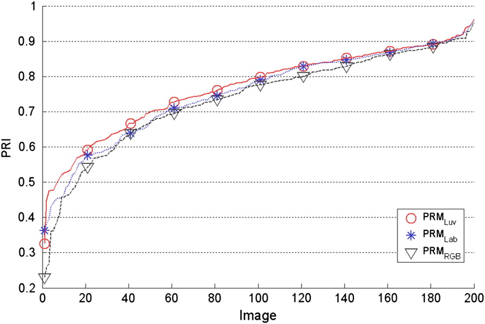

Fig. 5

Comparison of the Global Consistency Error (GCE) results of our approach in the three color spaces RGB, CIELab, and CIELuv. A low GCE value is desirable.

Fig. 6

Comparison of the Boundary Displacement Error (BDE) results of our approach in the three color spaces RGB, CIELab, and CIELuv. A low BDE value is desirable.

Table 2

Average performance and comparison in three color spaces using the 200 test images in the BSDS500.

	${\mathrm{PRM}}_{\mathrm{RGB}}$	${\mathrm{PRM}}_{\mathit{Luv}}$	${\mathrm{PRM}}_{\mathit{\text{Lab}}}$
PRI	0.738	0.768	0.754
Standard deviation PRI	0.142	0.120	0.132
$\mathrm{PRI}>0.7$ (# images)	137	150	143
GCE	0.229	0.205	0.219
BDE	12.50	10.72	10.87

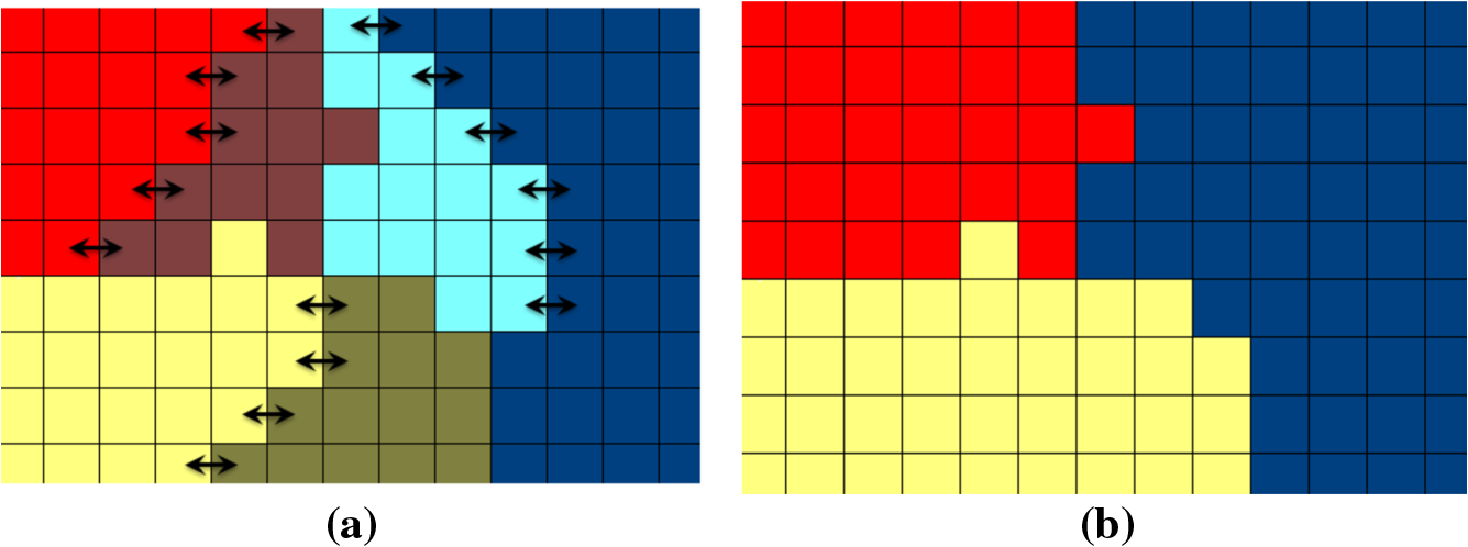
Note: The best performance for each measure is shown in bold.

Qualitative examples of the segmentation results using PRM are shown in Fig. 7. In each row, the original image and the corresponding outcome for each color space are visually compared. The original image is shown in the first row, while the resultant segmentation of the PRM using the RGB space is shown in the second row. The corresponding segmentations of the ${\mathrm{PRM}}_{\mathit{Luv}}$ and ${\mathrm{PRM}}_{\mathit{\text{Lab}}}$ are shown in the third and fourth rows, respectively. From this qualitative comparison, we can observe that the resulting segmentations of the perceptual spaces outperform the results using the RGB color representation. It can be seen that, in these examples, the outputs from the ${\mathrm{PRM}}_{\mathrm{RGB}}$ show a clear over-segmentation, and the ${\mathrm{PRM}}_{\mathit{Luv}}$ and ${\mathrm{PRM}}_{\mathit{\text{Lab}}}$ succeed in associating regions with similar colors.

Fig. 7

Qualitative comparison of three samples (first row) out of 500 images from the BSDS500 in the different color spaces under analysis (RGB in the second row and CIELuv and CIELab on the third and fourth rows, respectively).

4.2.

Performance Comparison with Other Methods

After the study of the PRM in different color spaces, a comparison of our approach in the CIELuv color space ${\mathrm{PRM}}_{\mathit{Luv}}$ against other rough set theory-based segmentation methods is conducted. The comparison is carried out with the roughness index-based technique (RBM)¹⁹ and the roughness approach through smoothing local difference (referred to as RSLD).²⁹ The RSLD method is of special interest, since it is a roughness index-based performed on the perceptual color space CIELuv. The results for the normalized cuts method (NCuts)³⁸ and the mean shift segmentation approach¹¹ are also included. The NCuts and mean shift methods are considered in this comparison because of their influence as widely used methods in image segmentation tasks. Besides, they are considered as de facto standard references for evaluation purposes. It is important to mention that the outcomes of the RBM and the RSLD methods were obtained with our implementation of the algorithms described by the authors. The outcomes from the NCuts and mean shift methods were obtained with publicly available code.

The average PRI, GCE, and BDE results for all methods, using the 300 images for training from BSDS500, are displayed in Table 3. From this table, we can see that the higher average value of 0.752 is achieved by ${\mathrm{PRM}}_{\mathit{Luv}}$, followed by the RBM with an average of 0.743. The lowest ${\mathrm{PRI}}_{\text{average}}$ is obtained with the RSLD method with 0.620. In this table, again, our method obtains more images with PRI values higher than 0.7. In this case, the approximation with the lowest standard deviation is the NCuts method with 0.119. However, our approximation is the second more precise method with a standard deviation of 0.133. In the case of GCE and BDE measures, the minor error values are attained by the ${\mathrm{PRM}}_{\mathit{Luv}}$.

Table 3

Average performance and comparison with other methods using the 300 training images in the BSDS500.

	${\mathrm{PRM}}_{\mathit{Luv}}$	RBM	RSLD	Mean shift	NCuts
PRI	0.752	0.743	0.620	0.653	0.722
Standard deviation PRI	0.133	0.135	0.176	0.204	0.119
$\mathrm{PRI}>0.7$ (# images)	219	180	114	141	200
GCE	0.203	0.302	0.230	0.270	0.298
BDE	11.42	15.75	15.18	11.98	14.05

Note: The best performance for each measure is shown in bold.

The corresponding results for the 200 test images in the BSDS500 were also obtained and compared. In Figs. 8, 9, and 10, the PRI, GCE, and BDE values, respectively, are plotted. We can observe from Fig. 8 that the ${\mathrm{PRM}}_{\mathit{Luv}}$ and mean shift corresponding results are very close on the top of the curves. It is interesting to notice that the NCuts curve in this figure records higher PRI values than the mean shift, RBM, and RSLD methods for the first 40 images and keeps its superiority over the RSLD method until image 90. Nevertheless, since the NCuts corresponding curve grows slowly, it drops below the rest of the algorithms from there on. The reason of this trend is that most of the resultant segmentations using NCuts attain a PRI value lower than 0.8 and that they tend to be very close to the mean of 0.722.

Fig. 8

Comparison of the PRI results of our method ${\mathrm{PRM}}_{\mathit{Luv}}$ with other rough set-based methods (RBM and RSLD) and reference methods (NCuts and mean shift) using the 200 test images from the BSDS500. A high PRI value is desirable.

Fig. 9

Comparison of the GCE results of the ${\mathrm{PRM}}_{\mathit{Luv}}$ with RBM and RSLD and the reference methods NCuts and mean shift using the 200 test images from the BSDS500. A low GCE value is desirable.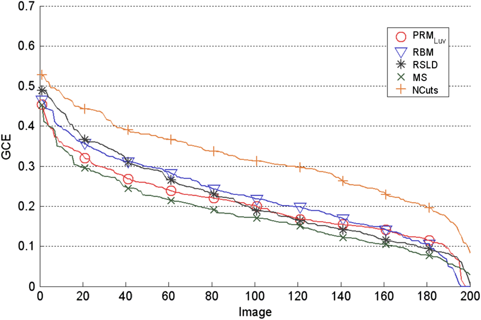

Fig. 10

Comparison of the BDE results of the ${\mathrm{PRM}}_{\mathit{Luv}}$ with RBM and RSLD and the reference methods NCuts and mean shift using the 200 test images from the BSDS500. A low BDE value is desirable.

In the case of Fig. 9, the curve with the lowest values is the one representing the mean shift approach and the curve with the highest errors is the NCuts one. It is difficult to make a visual separation of methods in Fig. 10, since the ${\mathrm{PRM}}_{\mathit{Luv}}$, RBM, RSLD, and mean shift curves are very close. The corresponding curve of the NCuts for the BDE measure is the only one that stands out from the rest of the curves, having the highest error values.

The averages of the quantitative measures for each method using the specific test set of images from the BSDS500 are shown in Table 4. For this set of 200 images, the higher PRI is achieved by the ${\mathrm{PRM}}_{\mathit{Luv}}$ with an average of 0.768, a standard deviation of 0.120, and 150 of the 200 images with a PRI value higher than 0.7. The second best is the mean shift method with a PRI average of 0.759 with a standard deviation of 0.148 and 137 images with a PRI value above 0.7. The lowest errors measured with the GCE and BDE are reached by the mean shift with 0.18 and the ${\mathrm{PRM}}_{\mathit{Luv}}$ with 10.72, respectively. In both cases, the largest errors are obtained by the NCuts. These errors occur because in the original method, the color image is processed using only the lightness component, hence ignoring the chromatic information.

Table 4

Average performance and comparison with other methods using the 200 test images in the BSDS500.

	${\mathrm{PRM}}_{\mathit{Luv}}$	RBM	RSLD	Mean shift	NCuts
PRI	0.768	0.734	0.707	0.759	0.708
Standard deviation PRI	0.120	0.147	0.154	0.148	0.098
$\mathrm{PRI}>0.7$ (# images)	150	138	117	137	137
GCE	0.205	0.224	0.217	0.180	0.317
BDE	10.72	12.61	13.88	11.02	14.01

Note: The best performance for each measure is shown in bold.

These results of the ${\mathrm{PRM}}_{\mathit{Luv}}$ indicates that this method has the best segmentation performance with high consistency and low error. In general, it is observed that the use of the proposed significant peaks selection, jointly with the merging strategy and the use of perceptual color spaces, improves the segmentation results with respect to the original proposal RBM. Moreover, the presented modifications allow better results in comparison with other classic segmentation methods in terms of the PRI measure.

5.

Conclusion

In this article, a set of modifications was proposed in order to improve a rough set theory-based segmentation method. This methodology takes advantage of the integration of spatial information about the pixels and the association of similar colors. The spatial information is added in two places: (1) within the histon representation, through the similarity computation of neighbor pixels, and (2) in the region-merging process, in which not only the similarity in the feature space is taken into account, but also the connectivity between two segments is considered. The proposed improvements are basically three. First, the use of perceptually uniform color spaces instead of the RGB color representation. From a quantitative evaluation, we have found that the CIELuv color space is the most suited representation for our specific segmentation method; meanwhile the CIELab space has a performance only slightly inferior. The use of a perceptual color representation allows our system to improve performance in the association of similar colors. The second improvement is an adaptive selection of the most suitable thresholds for a given image. The third one is the use of a region-merging process, which includes constraints about both spatial relation and color similarity, reducing over-segmentation problems. Experiments on an extensive database show that these modifications result in a method with better outcomes, outperforming other rough set theory–based approaches and classic reference segmentation algorithms.