Hardware validated unified model of multibit temporally and spatially oversampled image sensors with conditional reset

Thomas Vogelsang; David G. Stork; Michael Guidash

doi:10.1117/1.JEI.23.1.013021

13 February 2014 Hardware validated unified model of multibit temporally and spatially oversampled image sensors with conditional reset

Thomas Vogelsang, David G. Stork, Michael Guidash

Author Affiliations +

Journal of Electronic Imaging, Vol. 23, Issue 1, 013021 (February 2014). https://doi.org/10.1117/1.JEI.23.1.013021

Abstract

We describe a photon statistics-based theoretical model of the response to incident light of an image sensor and show that conditional reset and multibit temporal oversampling increase the dynamic range significantly. This photon-based modeling approach describes the full image sensor design space of temporal and spatial oversampling either with a binary comparison or with a multibit read of each sample. We find excellent quantitative agreement between measurements on custom hardware and our theoretical predictions. We then use this model to show what improvements in dynamic range and low-light response can be achieved by oversampling and what the limits of improvement caused by pixel size and lens parameters are.

1. Introduction

Over the past decade, CMOS image sensors have replaced both photographic film and CCD image sensors in nearly all imaging applications. During the same time, the advancement of silicon process technology according to Moore’s law has led to smaller and smaller pixels in many of these applications. In a conventional image sensor, a pixel is sampled only once per exposure. The high end of the dynamic range is therefore limited by the full well capacity of the pixel. The low end of the dynamic range is determined by the minimum amount of light required to generate a signal that can be distinguished from the combined photon noise and sensor read noise. Modern image sensors have achieved sensitivities of a few photo electrons.¹

The method proposed by us and other work discussed below apply oversampling to extend the dynamic range. In contrast to a conventional image sensor, an oversampling sensor combines multiple measurements of light intensity into a single pixel value of the final image. These multiple measurements can be distributed over space or over time or both.

To overcome the limitation of the high end of the dynamic range given by the reduced full well capacity and to make better use of highly sensitive pixels smaller than diffraction limit and with high sensitivity, Fossum²^,³ and Sbaiz et al.⁴ proposed oversampling the incident light in space and time, making a binary decision at each sampling event by comparing the number of detected photons against a threshold. The total number of photons can then be reconstructed from the results (0 or 1) of multiple such binary samplings. Yang et al.⁵ derived the theoretical limits of such binary oversampling based on photon statistics. All these proposals assume samplings equidistant in time and pixel reset after each sampling event and require a very small pixel with close to single-photon sensitivity. In the remainder of this paper, we will follow Ref. 3 by naming the binary sampled element “jot,” reserving “image pixel” or simply “pixel” for the aggregate that is used to form the final image. Vogelsang and Stork⁶ expanded this binary oversampling approach to be usable with less sensitive and conventional pixels and to provide more control over the sensor characteristics by the introduction of conditional reset and the variation of sampling thresholds and sampling interval durations. This new method fully resets the pixel instead of proportional to the sampled signal, and the threshold comparison and conditional reset is done at fixed times independent of the time when the threshold is reached. The sensor response is therefore different from $Σ Δ$ approaches (Refs. 7 and 8) to binary oversampling.

Multibit sampling differs from these binary oversampling approaches and has been shown to extend dynamic range as well. Many of today’s cameras have a high dynamic range (HDR) mode where multiple exposures with different exposure times are taken and afterward combined into a final image with extended dynamic range according to the proposal by Debevec and Malik.⁹ Extension of dynamic range in a single exposure can be achieved either by circuit techniques in the pixel that modify the effective full well capacity or by multiple samplings during light accumulation. Yang and El Gamal compared some of these approaches in Ref. 10. Multibit sampling at exponentially spaced time intervals employing a pixel-level analog-to-digital converter (ADC) has been further explored by Yang et al.¹¹ The sequence of effective sampling durations is monotonically increasing since there is no reset during an exposure. This limits the possibilities to shape the sensor response.

The conditional and selective per-pixel full reset of our proposed method allows sampling of each pixel with the optimum sample interval duration for the given illumination level without the need to add per-pixel decision circuitry or a pixel-level ADC. The only addition to a pixel is one transistor to enable column control of the reset in addition to the usual row control. The method is, therefore, well suited for sensors with small pixels.

Vogelsang et al.¹² have shown a fundamental equivalence between multibit oversampling of pixels and binary oversampling using virtual jots that have thresholds at the steps of the ADC. As such, the same mathematical description applies to these two apparently different approaches. The mathematical representation of these approaches can be used to optimize the design of oversampled image sensors both for the expected light conditions and for the hardware properties of the pixel technology that is available to manufacture the sensor.

The work presented here is organized as follows. Section 2 describes our photon-based sensor model. The analytical model combining the theory of binary sampling first presented in Ref. 6 and multibit sampling first presented in Ref. 12 is described in Sec. 2.1, and the Monte Carlo approach that is used when noise sources other than photon shot noise need to be considered is described in Sec. 2.2. Different sampling policies (sampling schedules and threshold settings) are compared in Sec. 2.3, and an experimental hardware validation of the model is shown in Sec. 2.4. We then discuss in Sec. 3 how the photon-based sensor model can be related to imaging situations in the real world by connecting scene illumination and camera parameters to the image sensor parameters (Sec. 3.1) and use this relationship to compare low light and dynamic range capabilities of conventional digital cameras and cameras using the proposed oversampling sensor (Sec. 3.2). Section 4 summarizes our work.

2. Photon Statistics-Based Sensor Model

2.1.

Analytical Model

The light intensity incident on a pixel of an image sensor is, in general, represented as a digital number of a certain bit depth. In a conventional image sensor, this bit depth is the bit depth of the ADC used to sample the photodetector response. The binary oversampling sensors discussed above achieve their total bit depth through the number of spatial and temporal binary samplings that are combined to form the signal in an image pixel. Multiexposure HDR derives most of its resolution through ADC bit depth but has some temporal oversampling (unconditional or hard reset between samples). The total image sensor design space can, therefore, be viewed as a three-dimensional space with the bit depth of the ADC and the amount of temporal and spatial oversampling as the axes. Figure 1 illustrates this concept and shows planes of constant total bit depth as well as the design space used by different sensors. Our theory accurately models all combinations of temporal and spatial oversampling as well as ADC bit depth.

Fig. 1

Image sensor design space. Binary oversampling methods lie on the plane spanned by the temporal and spatial oversampling axes, while conventional image sensors lie on the analog-to-digital converter (ADC) bit depth axis. Multiexposure high dynamic range lies on the plane spanned by the temporal oversampling and ADC bit depth axes. Our theory describes the full three-dimensional design space.

2.1.1.

Binary sampling

Sensor operation

Each image pixel comprises a number of binary sampled jots. At each sampling event, each jot produces a single binary output (a 1) if its integrated exposure exceeds a threshold $θ$ and a 0 otherwise. If the jot produces a 1, then its integrated exposure is reset to 0; otherwise its integrated photon signal is not reset (a nondestructive read), as shown in Fig. 2. The threshold in each binary jot can be varied in space or time to improve image quality.

Fig. 2

The dots on the $x$ axis indicate random photon strikes in a jot and the dot-dash line is their cumulative histogram. The vertical dashed lines show the sampling intervals of constant period $τ$ . In this example ( $θ = 12$ ), the conditional reset occurs three times— $t = 2 τ$ , $4 τ$ , and $7 τ$ , and thus the digital output is $y = 3$ .

Forward response model

The mathematical theory of operation of this sensor architecture is based on repeated conditional sampling from Poisson distributions.

An image pixel consists of $S$ jots that are oversampled $N$ times within one exposure. The image pixel response $Y$ is the sum of the jot sampling results and, therefore, a number between 0 and $N \cdot S$ (other models could be used as well). Jots are grouped by type where jots of a given type all have the same area and the same threshold. The basic relations between these variables are $S = \sum_{i = 1}^{n_{T}} s_{i}$ , $t_{\exp} = \sum_{m = 1}^{N} t_{m}$ , and $A = \sum_{i = 1}^{n_{T}} s_{i} a_{i}$ , where $S$ is the spatial oversampling, i.e., the number of jots in an image pixel, $n_{T}$ is the number of types of jots (different types have different thresholds or area or both), $s_{i}$ is the number of jots of type $i$ in an image pixel, $t_{\exp}$ is the exposure time, $N$ is the temporal oversampling, i.e., the number of readouts during exposure time $t_{\exp}$ , $t_{m}$ is the duration of sampling interval $m$ (denoted as $τ$ when constant), $A$ is the area of an image pixel, and $a_{i}$ is the area of jot of type $i$ .

Photons impacting the image sensor are distributed according to a Poisson distribution. The probability of observing $θ$ or more photons in a jot given an average incident photon number $λ$ is therefore

Eq. (1)

Q (λ, θ) \equiv \Pr [k \geq θ; λ] = 1 - e^{- λ} \sum_{k = 0}^{θ - 1} \frac{λ^{k}}{k!} .

Key to the calculation of the expected sensor response is the probability $p_{i, m}$ that a jot of type $i$ will be at or above threshold in sampling interval $m$ . This probability can be computed calculating forward from the first to the last sampling interval.

Eq. (2)

p_{i, 1} = Q (λ_{i, 1}, θ_{i, 1}),

Eq. (3)

p_{i, 2} = r_{i, 1} Q (λ_{i, 2}, θ_{i, 2}) + \sum_{n = 0}^{θ_{i, 2} - 1} \frac{λ_{i, 1}^{n} e^{- λ_{i, 1}}}{n!} Q (λ_{i, 2}, θ_{i, 2} - n) + \sum_{n = θ_{i, 2}}^{θ_{i, 1} - 1} \frac{λ_{i, 1}^{n} e^{- λ_{i, 1}}}{n!},

Eq. (4)

p_{i, m \geq 3} = r_{i, m - 1} Q (λ_{i, m}, θ_{i, m}) + \sum_{n = 0}^{θ_{i, m} - 1} P_{1, m - 1}^{(i, n)} Q (λ_{i, m}, θ_{i, m} - n) + \sum_{j = 1}^{m - 2} r_{i, j} \sum_{n = 0}^{θ_{i, m} - 1} P_{j + 1, m - 1}^{(i, n)} Q (λ_{i, m}, θ_{i, m} - n) + \sum_{n = θ_{i, m}}^{θ_{i, m} - 1} P_{1, m - 1}^{(i, n)} + \sum_{j = 1}^{m - 2} r_{i, j} \sum_{n = θ_{i, m}}^{θ_{i, m} - 1} P_{j + 1, m - 1}^{(i, n)} .

Here, $p_{i, m}$ is the probability to sample at or above threshold at a jot of type $i$ at sampling interval $m$ , $r_{i, m}$ is the probability to reset a jot of type $i$ at sampling interval $m$ , $λ_{i, m}$ is the average number of photons impacting a jot of type $i$ during sampling interval $m$ , and $θ_{i, m}$ is the sampling threshold of jot of type $i$ in sampling interval $m$ . The terms in Eqs. (3) and (4) denote the jots’ sampling and reset history. The first term is the probability that the jot has been reset in the directly preceding interval, so that at least the threshold number of photons are needed to accumulate again to sample at or above threshold in the following interval. The other terms denote sequences where no reset has occurred in the directly preceding interval. They are summarized in Table 1. Each term needs to be multiplied with the probability of its occurrence and summed over the combinatorial possibilities of photon combinations to reach it.

Table 1

Sampling sequence types in a jot.

$Q (λ_{i, m}, θ_{i, m})$	Pixel has been reset at sampling $m - 1$ and threshold is reached at sampling $m$ .
$P_{1, m - 1}^{(i, n)} Q (λ_{i, m}, θ_{i, m} - n)$	Pixel has never been reset before sampling $m$ and threshold is reached at interval $m$ by adding $n$ photons in interval $m$ .
$P_{j + 1, m - 1}^{(i, n)} Q (λ_{i, m}, θ_{i, m} - n)$	Pixel has been reset at sampling $j < m - 1$ and threshold is reached at interval $m$ by adding $n$ photons in interval $m$ .
$P_{1, m - 1}^{(i, n)}$	Pixel has never been reset before sampling $m$ and threshold is reached at interval $m$ without adding photons in interval $m$ because the threshold of sampling $m$ is $n$ photons lower than the number of photons at the end of sampling $m - 1$ .
$P_{j + 1, m - 1}^{(i, n)}$	Pixel has been reset at sampling $j < m - 1$ and threshold is reached at interval $m$ without adding photons in interval $m$ because the threshold of sampling $m$ is $n$ photons lower than the number of photons at the end of sampling $m - 1$ .

The term $P_{a, b}^{(i, n)}$ is the probability of a photon sequence of total $n$ photons distributed over the sampling intervals $a$ through $b$ in a way that the threshold is not reached in any sampling interval $a$ through $b$ and that the sensor is not reset after sampling. The intervals $a$ and $b$ denote any pair of sampling intervals with $a$ being less equal to $b$ . There are different equations to calculate $P_{a, b}^{(i, n)}$ depending on the sequence of thresholds and the reset operation (see below).

The expected value of the image pixel response is

Eq. (5)

E [Y] = \sum_{i = 1}^{n_{T}} (s_{i} \sum_{m = 1}^{N} p_{i, m}) .

Unconditional reset

In the case of unconditional reset (cf., Refs. 2 to 5), after each sampling $r_{i, m} = 1$ and $P_{a, b}^{(i, n)} = 0$ . Equation (5), therefore, becomes

Eq. (6)

E [Y] = \sum_{i = 1}^{n_{T}} [s_{i} \sum_{m = 1}^{N} Q (λ_{i, m}, θ_{i, m})] .

Conditional reset with thresholds constant over time

If the pixels are conditionally reset only if they are sampled at or above threshold (cf. Fig. 2), then $r_{i, m} = p_{i, m}$ and the full equations need to be used. As long as the thresholds do not vary in time, it is, however, possible to find a simplified expression for $P_{a, b}^{(i, n)}$ as only one threshold needs to be considered.

The third term of Eq. (3) and the fourth and fifth terms of Eq. (4) vanish since there is no change in threshold. The range of the sum over $n$ of the second term of Eq. (3) and the second and third terms of Eq. (4) from 0 to threshold minus one makes sure that $n$ is never at or above threshold. The probability of $n$ photons below threshold in the sampling intervals $a$ to $b$ becomes, therefore, simply the Poissonian probability of $n$ photons. Since the sum of Poissonian probabilities over expected photon numbers is the Poissonian probability of the sum over these expected photon numbers, the sampling sequence probability becomes

Eq. (7)

P_{a, b}^{(i, n)} = \frac{{(\sum_{k = a}^{b} λ_{i, k})}^{n} e^{- \sum_{k = a}^{b} λ_{i, k}}}{n!} .

Conditional reset with temporally variable threshold

The most complex calculation is for a sensor with thresholds varying over time where the pixels are conditionally reset only when they have been sampled above threshold. In this case, $P_{a, b}^{(i, n)}$ needs to be evaluated by examining the photon sequences in detail. The set $Ξ_{a, b}^{(i, n)}$ of photon sequences ${φ_{a} \dots φ_{b}}$ is the subset of all possible sequences of total $n$ photons that do not exceed the threshold at any sampling between intervals $a$ through $b$ . The elements $φ$ of the sequence are the photon numbers reaching the sensor at each interval of the sequence. For computational simplification, all thresholds between sampling event $a$ and $b$ can be replaced by a monotonic sequence giving the sequence $θ_{i, a}^{'} \dots θ_{i, b}^{'}$ with $θ_{i, a}^{'} \leq θ_{i, b}^{'}$ . Such a replacement is not necessary to calculate the sampling probabilities, but the time required to do the computation depends strongly on the number of photon sequences, and this simplification, therefore, reduces computation time. The sequence can be made monotonic since if a lower threshold would follow a higher threshold and the number of photons in that sequence would be between the high and low threshold, it would be above the low threshold and the sequence would therefore not be a sequence that satisfies the condition that the number of photons is below the threshold for all intervals from $a$ to $b$ . This allows replacing nonmonotonic $θ$ with monotonic $θ^{'}$ by replacing high thresholds with following low thresholds. The sequence is then reduced to one entry per threshold value to the sequence $θ_{i, a}^{*} \dots θ_{i, b}^{*}$ with $θ_{i, a}^{*} < θ_{i, b}^{*}$ , and the sampling sequence probability becomes

Eq. (8)

P_{a, b}^{(i, n)} = \sum_{{φ_{a} \dots φ_{b^{*}}} \in Ξ_{a, b^{*}}^{* (i, n)}} \prod_{l = a}^{b^{*}} \frac{λ_{i, l}^{* φ_{l}} e^{- λ_{i, l}^{*}}}{φ_{l}!} .

The set $Ξ_{a, b^{*}}^{* (i, n)}$ of photon sequences ${φ_{a} \dots φ_{b^{*}}}$ is the subset of all possible photon sequences that fulfill the conditions $\sum_{l = a}^{b^{*}} φ_{l} = n$ and $\sum_{l = a}^{k} φ_{l} < θ_{i, k}^{*}$ $\forall k \in [a, b^{*}]$ . The list of effective thresholds $θ_{i, k}^{*}$ fulfills the conditions $θ_{i, k}^{*} < θ_{i, k + 1}^{*}$ $\forall k \in [a, b^{*} - 1]$ , $θ_{i, b^{*}}^{*} = θ_{i, b}$ , $θ_{i, k}^{*} \in \underset{a \leq r \leq b}{\underset{︸}{{θ_{i, r}}}}$ $\forall k \in [a, b^{*}]$ , $θ_{i, r} \geq θ_{i, r + 1}$ $\forall r \in [a, b]$ , and $θ_{i, k}^{*} = θ_{i, b}$ . The photon count in the modified intervals is determined as $λ_{i, l}^{*} = \sum_{r = a}^{b} λ_{i, r}$ .

2.1.2.

Multibit sampling

Equivalence of multibit and binary sampling

The equivalence between binary oversampling and multibit oversampling can be shown by examining the probabilities of the ADC to return a specific data number $d$ . If the ADC sampling a pixel has as output a number between 0 and $n_{T}$ in a sampling interval, then the expected pixel response in that interval is the sum over all possible ADC output values multiplied with their probability

Eq. (9)

E [Y_{m}] = \sum_{i = 1}^{n_{T}} i \cdot \Pr_{ADC} [i; λ_{m}] .

Here, $Y_{m}$ is the image pixel response at sampling interval $m$ .

If the ADC has a step size of $d_{m}$ in the temporal oversampling interval $m$ , then the probability $\Pr_{ADC} [i; λ_{m}]$ to return data number $i$ in that interval given an average number of photons $λ_{m}$ is the probability to sample $i \cdot d_{m}$ or more photons minus the probability to sample $(i + 1) \cdot d_{m}$ or more photons.

Eq. (10)

\Pr_{ADC} [i; λ_{m}] = \Pr [k \geq i \cdot d_{m}; λ_{m}] - \Pr [k \geq (i + 1) \cdot d_{m}; λ_{m}] .

Assuming $n_{T}$ virtual jots with thresholds at multiples of the ADC step size $d_{m}$ in sampling interval $m$ , one can set the threshold $θ_{i, m}$ of the $i$ ’th virtual jot to

Eq. (11)

θ_{i, m} = i \cdot d_{m} .

It follows then from the definition of $p_{i, m}$ as the probability to sample at or above threshold at a jot of type $i$ at sampling interval $m$ together with Eq. (9).

Eq. (12)

E [Y_{m}] = \sum_{i = 1}^{n_{T} - 1} i [p_{i, m} (λ_{m}, i \cdot d_{m}) - p_{i + 1, m} (λ_{m}, (i + 1) \cdot d_{m})] + n_{T} p_{n_{T}, m} (λ_{m}, n_{T} \cdot d_{m}) = \sum_{i = 1}^{n_{T} - 1} i p_{i, m} (λ_{m}, i \cdot d_{m}) - \sum_{i = 2}^{n_{T}} (i - 1) p_{i, m} (λ_{m}, i \cdot d_{m}) + n_{T} p_{n_{T}, m} (λ_{m}, n_{T} \cdot d_{m}) .

Grouping the sums cancels the terms proportional to $i$ and leaves

Eq. (13)

E [Y_{m}] = \sum_{i = 1}^{n_{T}} p_{i, m} (λ_{m}, i \cdot d_{m}) = \sum_{i = 1}^{n_{T}} p_{i, m} (λ_{m}, θ_{i, m}) .

This is the expected value in sampling interval $m$ of a pixel consisting of $n_{T}$ binary sampled jots having thresholds according to Eq. (11), each jot receiving the average light intensity $λ_{m}$ corresponding to the light intensity impacting the multibit sampled pixel. Multibit oversampling is, therefore, equivalent to binary oversampling with virtual jots having thresholds at the steps of the ADC.

There are, however, important differences between virtual and real jots that need to be considered. Real jots need to be placed in different spatial positions, while the virtual jots of the multibit sampling all occupy the area of the image pixel. Hence, virtual jots are larger than real jots for any given pixel size. Because the virtual jot has a larger photoactive area, a multibit oversampled image sensor will have better low-light response than a spatially oversampled binary image sensor if all other factors such as sensitivity are held constant. Such a spatially oversampled image sensor can achieve the same low-light response only if it has jots that are more light-sensitive by a factor that compensates for the jot area reduction. Also, either all or none of the virtual jots that correspond to a pixel have to be reset, while a pixel using real jots and conditional reset would reset the jots above the threshold but not below the threshold. In Eqs. (3) and (4), a common reset threshold $r_{i, m} = θ_{r s t, m}$ has to be used when calculating reset probabilities. To calculate the final pixel response, ADC results are captured and summed up when the ADC is above the threshold and at a final residue read at the end of the exposure. The expected pixel response then becomes

Eq. (14)

E [Y] = \sum_{i = 1}^{n_{T}} \sum_{m = 1}^{N - 1} \frac{p_{θ_{r s t}, m}}{p_{1, m}} p_{i, m} + \sum_{i = 1}^{n_{T}} p_{i, N} .

2.1.3.

Sampling policies

The analytical model discussed above describes the sensor response as function of the selected oversampling type (binary or multibit, spatial, temporal, or both), the sequence of thresholds, the duration of temporal oversampling intervals, the area of the jots and pixels, and the reset conditions. We use the term “sampling policy” to describe the set of sampling periods, thresholds, and spatial areas of pixels comprising an image pixel. Different such policies will yield different response curves and noise characteristics. In an actual hardware sensor, some of the parameters can be varied in use while others are fixed at manufacturing. The selection of the right sampling policy defines the exposure setting of a sensor according to our proposal, similar to the selection of exposure time and ISO in a conventional sensor.

The achievable low end of the dynamic range is defined by the total exposure time, light sensitivity, and the noise level of the sensor. At very low light levels, no conditional reset will occur, and the sensor response will be the signal measured at the end of the exposure time proportional to all photons that have struck the pixel during that time. In multibit oversampling, a signal different from 0 will be reached if the ADC output is at least 1 data number. In spatial binary oversampling, the required condition is that at least one jot has reached or exceeded the threshold. The high end of the dynamic range on the other hand is defined by the duration of the shortest oversampling interval and the respective threshold and ADC step size used when sampling that interval. The measured signal will be meaningful, i.e., below saturation, if in the case of multibit oversampling the ADC output is at least 1 data number below its saturation or full well value and in the case of binary spatial oversampling if at least one jot has not reached the threshold.

2.2.

Monte Carlo Model and Sensor Noise

2.2.1.

Monte Carlo model description

The analytical model described above includes the full effect of photon shot noise since it is based on the Poisson statistics of the incident photons. A real image sensor also has intrinsic temporal and spatial noise sources that influence its response: read noise from the pixel read-out path, ADC noise, amplifier noise, and reset noise. Models for all these additional noise sources can be included in a Monte Carlo model of the sensor response.

The Monte Carlo model described here follows the approach of the analytical model by simulating Poisson distributed photons impacting the sensor, but it has models for the other noise sources listed in Table 2 added. Figure 3 shows the flow diagram of the Monte Carlo program. In the case of only temporal oversampling (either binary or multibit), there is only one real jot per pixel, so the expression “per real jot” in Fig. 3 can be read as “per pixel.”

Table 2

Sensor noise in Monte Carlo program.

Noise	Cause	Model
Fixed pattern noise	Random deviations of circuitry, e.g., threshold voltage variation. Can be per pixel or per circuit that is shared by a number of pixels, e.g., an analog-to-digital converter (ADC).	Number of photo electrons has the same adder each time it is sampled. The adder is done as random number from a normal distribution around 0 either per pixel or for a group of pixels. The fit parameter is the standard deviation.
Temporal threshold noise	Analog comparison to a threshold, e.g., by using a sense-amplifier, is subject to noise that can be different for different time intervals.	The threshold is modified according to a normal distribution around 0. The fit parameter is the standard deviation.
Pixel response nonuniformity	Pixel-to-pixel gain variation. Noise is proportional to light intensity, i.e., number of photo electrons.	The number of photo electrons to be sampled is multiplied by a random number according to a normal distribution around 1. The fit parameter is the standard deviation.
Read noise	Along the analog read path from pixel to ADC noise can change the sampled value.	The number of photo electrons is modified according to a normal distribution around 0. The fit parameter is the standard deviation.
Reset noise	Switching the reset transistor off changes the reset level (thermal switching noise)	The reset level is modified according to a normal distribution around 0. The fit parameter is the standard deviation.

Fig. 3

Flow diagram of Monte Carlo model.

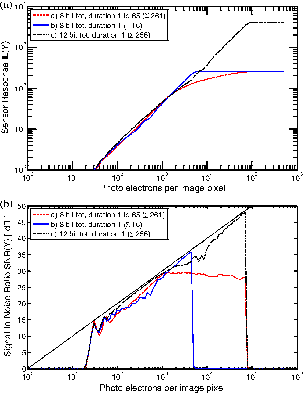
2.2.2.

Modeled noise sources

An image sensor has a number of noise sources that have to be included when one wants to accurately simulate its response. In the Monte Carlo model used in this work, we model the noise sources described in Table 2.

2.2.3.

Linearization of response

Image processing chains of typical imaging systems expect that the sensor output is a linear function of light intensity when they perform functions like color demosaicking or white balance. If the binary above-threshold counts or the ADC outputs at each above-threshold event are directly added to each other, then the sum is generally not linear. Linearization can be achieved by a number of methods. One method is to precalculate the expected response as a function of light intensity and then to use a lookup table to get the light intensity from a measured pixel response. Another method is to use a weighted sum that linearizes the response, instead of the simple sum over individual samples. If each response that is above the threshold and becomes part of the final response is weighted by the ratio of the time since the previous reset to the total exposure time, then the response becomes linear. Only nonsaturated ADC outputs can be used in this method. If all ADC outputs are saturated, then the response becomes the total exposure time divided by the shortest interval duration. Let $T_{i}$ denote the time since last reset before $Y_{i}$ , and the linear response becomes

Eq. (15)

Y_{linear} = {\begin{cases} \frac{t_{\exp}}{\min_{i \in 1 \dots N} t_{i}} Y_{sat} & Y_{i} = Y_{sat} \forall i \in 1 \dots N \\ \frac{t_{\exp}}{\sum_{i s. t. Y_{sat} > Y_{i} \geq θ_{r s t}} T_{i}} (\sum_{i s. t. Y_{sat} > Y_{i} \geq θ_{r s t}} Y_{i}) & \exists i s. t. 0 < Y_{i} < Y_{sat} \\ 0 & Y_{i} = 0 \forall i \in 1 \dots N \end{cases} .

Since the maximum possible result of Eq. (15) is larger than the saturated ADC output by a factor of the ratio of the total exposure time to the duration of the shortest sampling interval, while the direct sum has the saturated ADC output multiplied with the number of sampling intervals as maximum, the linearized response spans a wider numerical range than the direct sum if the sampling intervals are not of the same duration.

2.3.

Comparison of Sampling Policies

2.3.1.

Spatial, temporal, and multibit oversampling

Figures 4 (unconditional reset) and 5 (conditional reset) compare the different approaches. Lines denote the analytical model; symbols denote Monte Carlo simulation in the top graphs. The signal-to-noise ratio (SNR) shown in the bottom graphs is derived from Monte Carlo simulation. In all cases, the total bit depth is 8, and the various policies with temporal oversampling have variable sampling interval duration with the longest interval 128 times longer than the shortest to extend the dynamic range without increasing the total bit depth. The dotted black curve is the response of a conventional sensor with an 8-bit ADC and 20 electrons per data number saturating at 5100 electrons. The other curves are oversampling sensors, adding the result of the individual samplings. Gray curves are binary oversampling sensors with a threshold of 20 electrons. The dashed gray curve is of a sensor that oversamples only in time (256 times), while the solid gray curve oversamples both in space (16 jots) and time (16 times). The black dot-dash curve is a sensor oversampling in time (16 times) with a 4-bit ADC.

Fig. 4

Response (a) and signal-to-noise ratio (b) when using unconditional reset. All curves have a total bit depth of 8. The binary oversampled methods have the worst low-light response, followed by the temporally oversampled multibit method. None of the oversampled methods reaches the low-light response of the conventional sensor, but all extend the dynamic range at the high end.

Fig. 5

Response (a) and signal-to-noise ratio (b) when using conditional reset. All curves have a total bit depth of 8. The temporally oversampled methods have the same low-light response as the conventional sensor, but extend the dynamic range at the high end. Only the spatially oversampled method has less low-light response.

All sampling policies shown in Fig. 4 reset the pixel after each sampling. Without conditional reset, binary temporal and mixed temporal and spatial oversampling is equivalent (gray curves in Fig. 4). The bright-light response is extended for the binary sampling approach compared to that of the conventional sensor readout. The low-light response of the binary pixel without conditional reset is much worse than the conventional (black dotted curve) approach since the number of photons per jot and sampling interval is lower. The multibit temporal oversampled pixel (dot-dash black curve) has improved low-light response since the spatial oversampling is less.

Figure 5 shows the improved low-light response when conditional reset is used. The colors and line styles of the different curves correspond to the same sampling policies as in Fig. 4. Unlike the case shown in Fig. 4, pixels are reset only if they are sampled at or above the threshold (binary oversampled gray curves) or if the data number returned by the ADC is not zero (multibit oversampled black dot-dash curve). The only curve that shows reduced low-light response corresponds to the approach with spatial oversampling (solid gray curve). The temporally oversampled approaches keep the extended bright-light response. As a result of retaining low-light response and extending the bright-light response, the sensor dynamic range is extended. In this example, the dynamic range is extended by a factor of 20 compared to a conventional sensor, corresponding to an increase of effective full well capacity from 5100 electrons to over 100,000.

2.3.2.

Threshold sequencing

Figure 6 shows a comparison of threshold sequences. The ascending binary oversampled threshold sequence of Fig. 6(a) will have a reduced low-light response compared to the descending sequence of Fig. 6(b) but an increased high end of the dynamic range. The reason is that the low-light limit of the dynamic range is reached when no intermediate conditional reset has occurred and the light collected over the full exposure time is assessed with the last threshold and readout. Since that last threshold is higher for an ascending sequence, such a sequence will have a reduced low-light response. The high end of the range is determined by a combination of threshold and sampling interval duration. In Fig. 6(a), the shortest interval has also the highest threshold and will, therefore, have the highest end of the dynamic range. Figure 6(c) shows the virtual jots when using multibit oversampling. Since the ADC steps are always present, both low and high thresholds are always present as well, and thus the wide dynamic range leads to both a good low-light response and a high limit in bright illumination.

Fig. 6

Sampling policies with different threshold sequences. The dynamic range of the binary oversampled ascending sequence (a) will be shifted to higher light intensities compared to the descending sequence (b) since the bright-light response is determined by the threshold in the shortest interval, while the low-light response is determined by the threshold at the end of the exposure time when conditional reset is used. When using multibit oversampling, all thresholds are present in the virtual jots (c) at all intervals, and the response spans the widest range.

2.3.3.

Variation of interval duration

Figure 7 compares three different sampling policies. The response is shown on top and the SNR on the bottom. All policies use multibit oversampling with a 4-bit ADC and a full well capacity of 300 electrons. The first two policies temporally oversample 16 times for a total bit depth of 8 bits. The first curve [(a), red dashes] varies the sampling interval duration logarithmically from 1 to 65 relative to each other so that the shortest interval is 1/261 of the total exposure time. This number was picked to be as close as possible to the equidistant ratio of the third curve with logarithmically spaced integer thresholds. The second curve [(b), solid blue] has intervals of equal length, each interval being $1 / 16$ of the total exposure time. The third curve [(c), black dot-dash) again uses equidistant temporal oversampling, however, with 256 samples for a total bit depth of 12 bits. The dynamic range of the policies with similar length of the shortest interval [(a) and (c)] is nearly the same, while the dynamic range of the approach with longer intervals (b) is much less. The SNR curves show that the price of achieving high dynamic range with fewer samplings is a reduced SNR at the high end. The response with equal sampling intervals stays close to linear and the SNR follows the photon shot noise limit, while the approach with varying interval duration has a response that shows quasi-logarithmic behavior and the SNR saturates.

Fig. 7

Response (a) and signal-to-noise ratio (b) of policies with constant and variable interval duration. Variable interval duration can extend the dynamic range to be as large as when using a much higher total bit depth at the cost of a reduced signal-to-noise ratio at the high end.

2.4.

Hardware Verification

We compared our sensor model to hardware on a small test chip and presented initial results in Vogelsang et al.¹² The results shown here are from later measurements of the same hardware. The pixel is based on a conventional 4T-pixel to which an additional transistor is added to provide column control in addition to row control for pixel reset. The test chip was built in a 180 nm CMOS image sensor technology using a fully pinned photodiode and a pixel pitch of 7.2 μm. The measured conversion gain is $83 μ V / e^{-}$ . The read noise was fitted as $10 e^{-}$ and the photoresponse nonuniformity as 1.5%. The pixel was oversampled four times with a 10-bit ADC, and the ratio of the shortest interval to the total exposure time was $1 ∶ 13$ .

Figure 8 shows a comparison of the simulated and measured response, and Fig. 9 shows the same comparison for the SNR. Linearization was done according to Eq. (15). The dashed and solid lines denote the simulated curves for conventional and oversampled operations, respectively, while the asterisks and circles, respectively, denote the corresponding measurement results. The agreement between measurement and simulation is very good. At an SNR of 0 dB, the dynamic range is 58 dB for the conventional operation and 79 dB for the oversampled operation. At an SNR of 20 dB, the dynamic range is 35 and 56 dB, respectively. The sampling policy chosen for this example did, therefore, expand the dynamic range by 21 dB or a factor of 11.

Fig. 8

Model-to-hardware comparison of the response of an image sensor operated conventionally, respectively, oversampled with conditional reset. The response of the oversampled sensor was linearized using the weighted sum of Eq. (15).

Fig. 9

Model-to-hardware comparison of the signal-to-noise ratio of the linearized response of an image sensor operated conventionally, respectively, oversampled with conditional reset. The dynamic range is extended by 21 dB.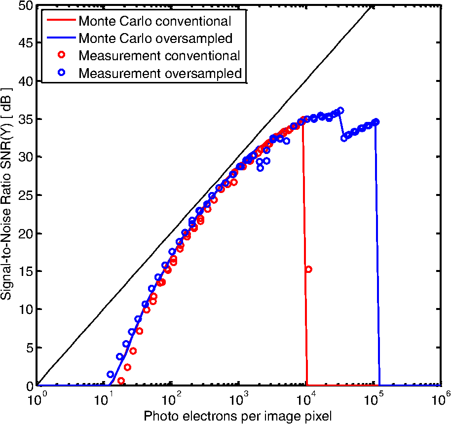

The SNR of the oversampled sensor shows a clearly visible dip in the extended dynamic range part of the curve. This dip is caused by not having identical duration of all subframes. In the measurement and simulation shown here, the first subframe had one quarter of the duration of the other three subframes. When subframes of similar duration are combined with oversampling with conditional reset, the dynamic range is extended with a smooth continuation of the SNR curve (here from $\sim 10^{4}$ photo electrons to $\sim 3 \cdot 10^{4}$ photo electrons). The shorter subframe, however, creates an SNR curve that is shifted according to the duration ratio. Combining this short subframe with the other three subframes extends the dynamic range further to $\sim 1.2 \cdot 10^{5}$ photo electrons, but the SNR is lower when there are so many photons that the longer subframes saturate. When designing the sampling policy for the sensor, it is important to make sure that such a dip does not extend below a desired SNR in order to not visibly degrade the image. In this example, the lowest point of the dip is over 30 dB, which will still give a very good image quality.

3. Camera Parameters and Sensor Modeling

3.1.

Scene Illuminance and Photons Per Pixel

The sensor model described so far relies on the knowledge of the number of photo electrons per pixel to calculate the sensor response. When one wants to predict the sensor response when taking images with a camera, the illuminance of the scene has to be translated into the number of photo electrons sampled by each pixel.

3.1.1.

Photon energy and illumination

To derive the number of photons impacting a pixel, it is first necessary to calculate the number of photons impacting a target area of which a camera is taking a picture of as a function of the specified illumination of that area.

The CIE spectral power density and luminosity curves¹³ can be used to calculate the number of photons for a given illuminant. The luminous flux per Watt for the spectrum of the illuminant is the product of the luminosity function $L$ and the spectral power density $D_{P}$ integrated over the visible spectrum. By integrating the spectral power density of the illuminant over the wave length, average photon energy for the illuminant can be derived as well. Together these calculations give the number of photons that impact a given area $a_{target}$ during the exposure time at a given illuminance $E_{V}$ as

Eq. (16)

\tilde{Λ} = γ E_{V} t_{\exp} a_{target} .

Here, $\tilde{Λ}$ is the average number of photons incident on an image pixel during the exposure time $t_{\exp}$ and $γ$ is the photon density.

The constant $γ$ that gives the number of photons per luminous energy and area is dependent on the illuminant. For the standard daylight spectrum CIE-D65, this constant is

Eq. (17)

γ_{D 65} = 12612 {lx}^{- 1} {μ m}^{- 2} s^{- 1} .

For a spectrum that is shifted to longer wavelengths, the number of photons is higher for two reasons: (1) such a spectrum is not centered on the peak eye sensitivity; there is, therefore, more power needed for one lumen and (2) long-wavelength photons are less energetic, and therefore, more such photons are needed to provide a given power. For the standard incandescent spectrum CIE-A, the constant is

Eq. (18)

γ_{A} = 19892 {lx}^{- 1} {μ m}^{- 2} s^{- 1} .

3.1.2.

Lenses and pixel size

The previous section related the illuminance of the target to the number of photons impacting that target. As a next step, the fraction of these photons that reach a pixel of the image sensor needs to be calculated. Assuming Lambertian reflection of the target and a lens focused at infinity, the illuminance of the sensor can be calculated from the illuminance of the target.

Multiplying with the quantum efficiency as the factor between the number of photons and the number of converted photo electrons gives an expression similar to the one derived in Ref. 14 that allows calculation of the number of photons sensed by an image pixel as a function of target illuminance, target reflectivity, the f-number of the lens, the exposure time, and the pixel area with

Eq. (19)

Λ = Q E \cdot γ \frac{1}{4} \frac{ρ}{F^{2}} E_{V}^{target} t_{\exp} A .

Here,

Λ

is the average number of photons sensed in an image pixel during the exposure time

t_{\exp}

, QE is the quantum efficiency,

ρ

is the reflectivity, and

F

is the f-number.

3.2.

Low-Light and Dynamic Range Capabilities

3.2.1.

Influence of pixel size and lens

The simulations whose results are shown in Fig. 10 apply Eq. (19) to generate the number of photons as input for the sensor model based on target illumination. Compared are three different sensing schemes: the first is the conventional single-shot approach, the second is a dual-shot HDR approach, where the ratio between the short and long exposure is $1 ∶ 4$ , and third is the oversampled approach proposed in this work. In all oversampled curves, the incident light is oversampled four times with intervals of relative sampling durations 1, 2, 4, and 8. At the lowest light intensity, no conditional reset occurs and the response is that of a conventional sensor, while at highest intensity, the pixel is above the threshold and, therefore, resets every time, and the shortest sampling interval becomes 1/15 of the exposure time.

Fig. 10

Signal-to-noise ratio as function of scene illumination: (a) mobile sensor and (b) DSLR sensor. In both cases, a comparison at the low-light and at the bright-light end is shown. At the low-light end, the same total exposure time is used for the conventional and oversampled operation to match the low-light response, while at the high end, a longer exposure time is used for the oversampled operation to extend the dynamic range to the low end while matching the bright-light response.

The spectrum of the illumination used in the simulation was D65. If a color filter array were present, one would integrate the spectral density function of the light source with the photopic response, the quantum efficiency, and the spectral response of each of the three color filters. To simplify the task, we used here a combined quantum efficiency of 40% for the pixel and color filter together with the integral over spectral density function and photopic response. It was possible to use this approach as we only want to compare the impact of pixel parameters and optics on the light sensitivity, not simulate a specific hardware solution. We used a target reflectivity of 18% for the simulations.

Figure 10(a) shows the simulated SNR of a small-pixel sensor typical for a mobile system. We assumed a pixel pitch of $1.1 μ m$ and a fixed f-number of f/2.8. The full well capacity was assumed to be 5000 electrons and a 10-bit ADC was used. The exposure time of the conventional sensor (red curves) in a low-light situation (dashed lines) was assumed to be $1 / 15 s$ , close to the limit that can be done with a handheld camera. At the high end (solid lines), $1 / 2000 s$ of exposure time gives a high end of the dynamic range that is sufficient to take images in bright sunlit outdoor scenes. The oversampled sensor (black curves) uses the same exposure $1 / 15 s$ setting for the low-light situation, but increases the total exposure time for the bright-light situation to $1 / 200 s$ . The dynamic range is extended by 24 dB in both situations. At the low-light situation, this extension occurs at the high-intensity end. At the bright-light situation, our choice of exposure parameters extends the dynamic range mostly to the lower end.

Figure 10(b) shows similar results for a digital single lens reflex camera (DSLR)-type sensor. The assumed pixel pitch was $6.3 μ m$ , the f-number was variable between f/1.4 and f/22, the full well capacity was 50,000, and a 14-bit ADC was used. The extension of the dynamic range is similarly 24 dB between a conventional and our proposed oversampled sensor since the sampling policy is the same. As in the example of the mobile sensor, we selected an increased exposure time for the bright situation to extend the dynamic range to the lower end.

Figures 10(a) and 10(b) clearly show that the DSLR can cover a much wider total dynamic range than the mobile sensor. The extension of the dynamic range at the low end comes mainly from the large pixel area that accepts many more photons into a pixel according to Eq. (19). The larger aperture that is possible with DSLR lenses contributes as well. At the high end, the ability to make the aperture very small together with a shorter minimum exposure time extends the range.

It is also clear that the multibit oversampling with conditional reset approach provides a small pixel mobile camera system with very wide dynamic range and wide exposure latitude. A mobile camera system using this approach can expose for the low-light regions of the scene while retaining all of the bright-light information and detail.

Both SNR curves show a nonmonotonic behavior at high intensities. This is caused by the varying duration of the sampling intervals similar to Fig. 9. Figure 9 had only two different durations and, therefore, only one visible dip, while in Fig. 10, all four durations are different and there are three visible dips. Both for the mobile sensor and the DSLR, the dips occur above 30 dB SNR and will, therefore, not be visible on the final image.

The ability of the dual-shot approach (blue curves) to capture a wide dynamic range is as expected between the single-shot approach and our method. The nonmonotonic dip of the SNR curve in the dual-shot approach is more pronounced than in our approach since there are only two possible exposure times available, while in our approach, the conditional reset makes available all combinations of interval durations between the shortest interval length and the full exposure time. The dual-shot approach shows a slightly reduced SNR at the low-light end since we assumed that the sum of the short and long exposures is the same for all three methods compared, thereby making the long exposure shorter than both the total exposure time in our approach and the exposure time of a single shot.

3.2.2.

Optimization of low-light response

Figure 11 shows the response and SNR of the small-pixel sensor of Fig. 10(a) for different full well capacity and read noise. Since the dynamic range of the oversampled method is so much higher, the full well capacity can be reduced, in this example, from 5000 to 1250 electrons to shift the response curve to lower light intensities while still increasing the dynamic range at high light intensity. If the reduced full well capacity can be used to reduce the read noise as well, e.g., by a higher conversion gain, then the SNR at low light intensities can be improved compared to the conventional sensor.

Fig. 11

Comparison of response (a) and signal-to-noise ratio (b) of conventional and oversampled image sensors. The full well capacity of the conventional sensor is 5000 electrons. The oversampled sensor has 1250 electrons full well capacity and is oversampled four times with relative sample interval durations of 1, 2, 4, and 8. If the reduced full well capacity can be used to reduce the read noise, then the low-light response can be improved.

Figure 12 demonstrates this using the example of an image with 96 dB dynamic range. The top set of images is false color, comparing the quality of the reconstruction by showing the relative difference between the reconstructed linearized response and the original input data. The bottom set of images shows tone mapped simulation output. Identical tone mapping has been applied to all simulations. The small-pixel conventional sensor simulated in Fig. 10 is shown with two exposures, one optimized for the darker parts of the image (a) and one for the brighter parts of the image (b). The difference between the two exposures is two stops. The first exposure has overexposed highlights, while the second has significantly increased noise in the dark regions. The oversampled image (c) has reduced full well capacity (from 5000 to 1250 electrons) and sensor read noise (from 5 to 1 electron). The sequence of relative sampling durations was chosen to be 1, 2, 4, 8, 16, and 32 to match the large dynamic range of the input image. The total exposure is the same as for image (a). The oversampled approach gives even better bright-light reconstruction as the short exposure with the conventional sensor and excellent reconstruction of the dark parts of the image as well.

Fig. 12

False color (top) and tone mapped (bottom) output of an image simulation comparing conventional and oversampled sensors. The false color image shows the relative difference between the original and reconstructed linear response. The two left images (a) and (b) are calculated from the simulated response of the small-pixel conventional sensor used in Fig. 10; the right image is calculated from the simulated response of the oversampled sensor with reduced full well capacity and read noise. Different from Fig. 1, the sensor has been oversampled six times with relative sample interval durations of 1, 2, 4, 8, 16, and 32. Images (a) and (c) are exposed at the same exposure value, while image (b) is exposed at a two stops higher exposure value. The conventional sensor has either blown out highlights (a) or increased noise in the dark areas (b), while the oversampled sensor has high-quality reconstruction over the full dynamic range.

Figure 13 is another example comparing different HDR approaches. In this case, the four images compare a conventional single-shot exposure, the line-interleaved HDR approach in which alternating pairs of rows are exposed with different exposure times, dual-shot HDR blending two images with different exposure time, and the oversampling approach with conditional reset proposed in this work. The relative sample interval durations of our approach are 12, 1, 1, 1 in this example. Again, exposure values have been selected to get the best overall image quality in all cases. The exposure value of the line-interleaved and dual-shot HDR are, therefore, one stop higher than single shot, and the image taken with our approach is exposed three stops more. The line-interleaved image has a ratio of $2 ∶ 1$ between the long and short exposures, while the dual-shot image has a ratio of $4 ∶ 1$ . A comparison of the images clearly shows the benefit of our approach. The single-shot image is worst with saturated highlights and significant noise in the dark. The line-interleaved approach has better highlights, but the noise in the dark gets even worse due to the necessary interpolation. Dual shot does not have this problem and has both better exposed highlights and less noise, but it is still significantly noisier than our approach.

Fig. 13

Full image (top) and zoom into dark part (bottom) of a high dynamic range image. The exposure has been adjusted to take advantage of wider dynamic range; line interleaved and dual shot are therefore exposed one stop more than the single-shot image, and the oversampling with conditional reset of this work is exposed three stops more than the single-shot image.

4. Conclusions

We have developed a theoretical model that describes light capture of a photosensor based on photon statistics, thereby incorporating photon shot noise directly. This model describes the sampling of photons as a series of binary comparisons with a threshold. We showed in previous work that multibit sampling with an ADC is mathematically equivalent to spatially oversampling the pixel with virtual jots that are sampled with thresholds at the steps of the ADC. Our sensor model can, therefore, be used to predict and optimize the light response of any binary oversampling sensor, conventional single-sample multibit sensors, and multibit oversampling sensors. The sensor response can be linearized either by a lookup table or by a weighted sum of the results of the individual samplings. We verified this model on hardware using a small test chip. Using the model, we demonstrated that sampling policies that use only temporal oversampling (binary or multibit) and reset the pixel only conditionally when a threshold has been reached have better low-light response than sampling policies with unconditional reset or spatial oversampling. By calculating the number of photons on the sensor based on target illumination and camera parameters, we were able to compare exposure settings for low-light and bright-light settings of conventional sensors with oversampled sensors both for sensors typical for mobile devices as for DSLR sensors. A significant increase of dynamic range of $\sim 24 dB$ in our example can be seen in all cases. In a typical camera application, the dynamic range would be extended to the high end in a low-light situation and to the low end in a bright-light situation. The dynamic range of an oversampled mobile camera can be as large as the range of a conventional DSLR in medium- or bright-light situations. Such a matchup is not possible either at very low light situations where the pixel size is important to collect as many photons as possible or at very bright light situations where the aperture needs to be changed to let less light on the sensor. While the high end can be further extended in all cases by more oversampling, at the low end, an improvement is only possible when more photons can be collected by having a larger pixel area, higher pixel sensitivity, or a combination of these approaches. We expect that the pixel can be designed to achieve higher sensitivity when using our approach as there is no need to have a large full well capacity to handle brightly lit parts of the scene. More generally, low-light response can be improved in camera systems employing sensors having multibit oversampling with conditional reset by exposing for the low-light regions of the scene while retaining all of the bright-light information and detail.

References

1.

P. SeitzA. Theuwissen, Single-Photon Imaging, Springer, Berlin, Heidelberg (2011). Google Scholar

2.

E. Fossum, “What to do with sub-diffraction-limit (SDL) pixels,” in IEEE Workshop on Charge-Coupled Devices and Advanced Image Sensors, –217 (2005). Google Scholar

3.

E. Fossum, “The quanta image sensor (QIS): concepts and challenges,” in 2011 OSA Topical Meeting on Optical Sensing and Imaging, (2011). Google Scholar

4.

L. Sbaizet al., “The gigavision camera,” in IEEE Conf. on Acoustics, Speech and Signal Processing, 1093 –1096 (2009). Google Scholar

5.

F. Yanget al., “Bits from photons: oversampled image acquisition using binary Poisson statistics,” IEEE Trans. Image Process., 21 (4), 1421 –1436 (2012). http://dx.doi.org/10.1109/TIP.2011.2179306 IIPRE4 1057-7149 Google Scholar

6.

T. VogelsangD. G. Stork, “High-dynamic-range binary pixel processing using non-destructive reads and variable oversampling and thresholds,” in IEEE Sensors, 1 –4 (2012). Google Scholar

7.

S. KavusiH. KakavandA. El Gamal, “Quantitative study of high-dynamic range SigmaDelta-based focal plane array architectures,” Proc. SPIE, 5406 341 –350 (2004). http://dx.doi.org/10.1117/12.548875 PSISDG 0277-786X Google Scholar

8.

Z. IgnjatovicD. MaricicM. F. Bocko, “Low power, high dynamic range CMOS image sensor employing pixel level oversampling—analog-to-digital conversion,” IEEE Sensors J., 12 737 –746 (20122012). http://dx.doi.org/10.1109/JSEN.2011.2158818 ISJEAZ 1530-437X Google Scholar

9.

P. DebevecJ. Malik, “Recovering high dynamic range radiance maps from photographs,” in Proc. of 24th Annual Conf. on Computer Graphics and Interactive Techniques, 369 –378 (1997). Google Scholar

10.

D. YangA. El Gamal, “Comparative analysis of SNR for image sensors with enhanced dynamic range,” Proc. SPIE, 3649 197 –211 (1999). http://dx.doi.org/10.1117/12.347075 PSISDG 0277-786X Google Scholar

11.

D. Yanget al., “A 640 x 512 CMOS image sensor with ultrawide dynamic range floating-point pixel-level ADC,” IEEE J. Solid-State Circuits, 34 (12), 1821 –1834 (1999). http://dx.doi.org/10.1109/4.808907 IJSCBC 0018-9200 Google Scholar

12.

T. VogelsangM. GuidashS. Xue, “Overcoming the full well capacity limit: high dynamic range imaging using multi-bit temporal oversampling and conditional reset,” in International Image Sensors Workshop, (2013). Google Scholar

13.

“CIE standard colorimetric observer data and CIE standard illuminant data,” http://www.cis.rit.edu/mcsl/online/cie.php Google Scholar

14.

J. Alakarhu, “Image sensors and image quality in mobile phones,” in Int. Image Sensors Workshop, (2007). Google Scholar

Biography

Thomas Vogelsang received his diploma and doctoral degree in physics from the Technical University Munich. He worked on DRAM from 1994 to 2009 at Siemens, Infineon, Qimonda, and Rambus. Since 2010 he has been a member of the Computational Sensing and Imaging group of Rambus Labs and leading the work on binary pixels. He is a senior member of the IEEE, and author or co-author of 14 publications, 20 patents and over 30 pending patent applications.

David G. Stork is Rambus Fellow and leads the Computational Sensing and Imaging Group within Rambus Labs. A graduate in physics from MIT and the University of Maryland, he has held faculty positions in eight disciplines in several leading liberal arts and research universities. His published eight books/proceedings volumes variously translated into four languages. He holds 43 patents and is a fellow of the International Association for Pattern Recognition and SPIE.

Michael Guidash received his BS in electrical engineering from the University of Delaware, and MS in electrical engineering from Rochester Institute of Technology. Michael worked at Kodak from 1981 to 2011 in the fields of CCD and CMOS image sensors. He led the R&D and product development of CMOS sensors. He is now consulting in CMOS sensor technology. He is an author or co-author of 15 publications, 69 patents and over 20 patent applications.

CC BY: © The Authors. Published by SPIE under a Creative Commons Attribution 4.0 Unported License. Distribution or reproduction of this work in whole or in part requires full attribution of the original publication, including its DOI.

Citation Download Citation

Thomas Vogelsang, David G. Stork, and Michael Guidash "Hardware validated unified model of multibit temporally and spatially oversampled image sensors with conditional reset," Journal of Electronic Imaging 23(1), 013021 (13 February 2014). https://doi.org/10.1117/1.JEI.23.1.013021

Published: 13 February 2014

Access the abstract

JOURNAL ARTICLE
14 PAGES

DOWNLOAD PAPER SAVE TO MY LIBRARY