|
|
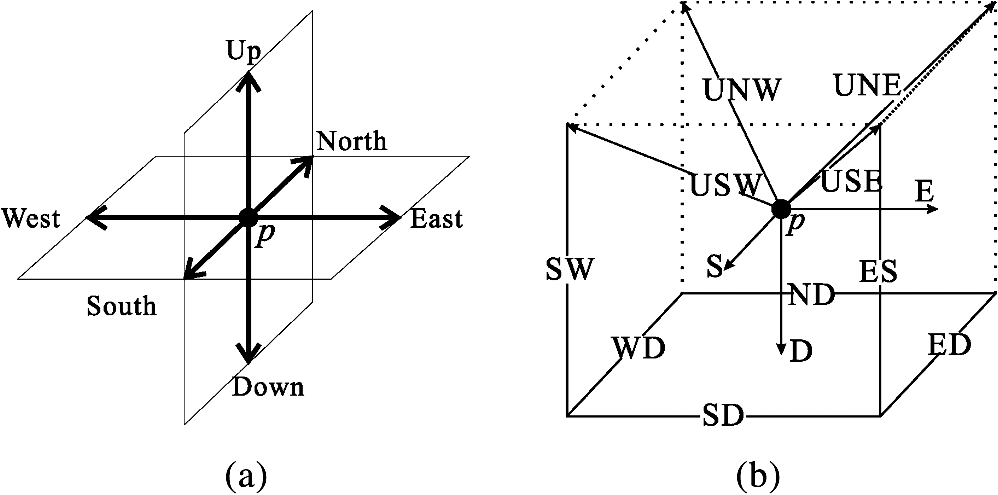
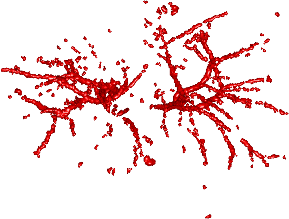
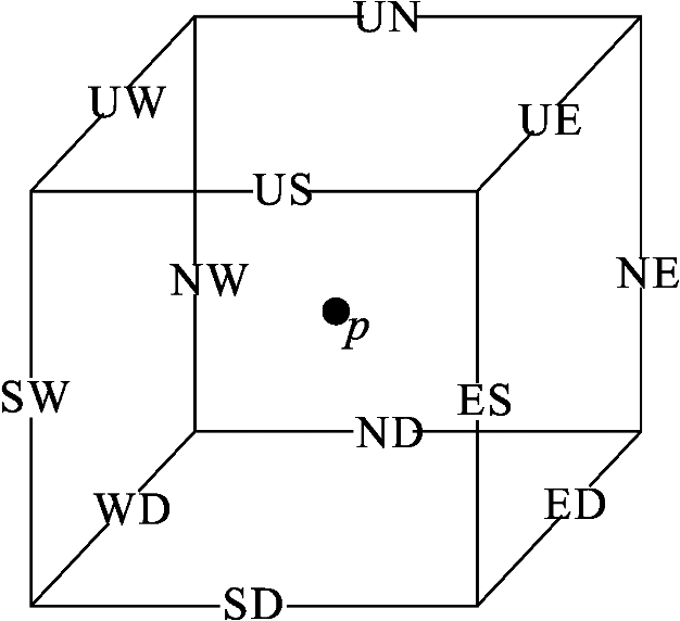
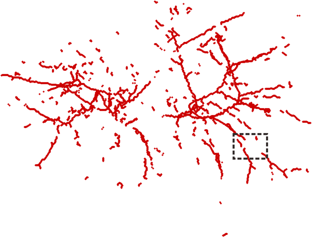
1.IntroductionVessel centerline has been used in computing edge gradients and searching for border positions,1 to derive video-densitometric profiles,2 for measurement of vessel diameter,3 for calculation of lesion symmetry,4 and as the basis for three-dimensional (3-D) reconstruction of vessel segments or of the entire arterial tree.3,5 Many techniques in the literature propose to detect vessel centerline by thinning algorithm.6–8 These algorithms are notoriously sensitive to noise and can result in ambiguous results at bifurcations. The results will lead to inaccuracies in width, vessel direction, and touristy measurements. Several articles have introduced tracking-based techniques for extraction of the vessel centerlines.9–12 In these approaches, vessel centerlines are extracted segment-by-segment while the vessel boundary associated with each segment is delineated. These algorithms require user intervention to determine the seed point. The axial tangent of the seed is then generated. This tangent helps to define a cross-sectional plane (normal plane) by shifting forward the current one along the tangential direction, on which the vessel is segmented and the next axial point is calculated as the centroid of the planar segmentation. This process keeps iterating until a termination criterion is met or the user preempts the tracing. In most images, however, noise and low-contrast pose significant challenges to the extraction of vessel centerline. For example, the central intensity of some vessels differs from the background by as little as 3 gray levels, yet the background noise standard deviation is 2.3 gray levels. Narrow vessels (in diameter ) often have the lowest contrast. In these cases, a disconnected vessel centerline may be obtained and, more importantly, the aforementioned methods9–12 may only produce an incomplete extraction of the vessel centerline. Some authors attempt to overcome these problems by improving vessel tracking.13–17 For example, Manniesing et al.15 presented an approach for vessel centerline tracking based on surface evolution. In this work, the main idea is to guide the evolution of the surface by analyzing its skeleton topology during evolution. Friman et al.16 proposed a multiple hypothesis template tracking approach for the segmentation of small 3-D vessel structures. This work also contributes a novel mathematical vessel template model, with which an accurate vessel centerline extraction is obtained. Wong and Chung17 proposed a probabilistic framework for vessel centerline tracing. In order to obtain a satisfactory vessel centerline extraction with the above methods, user guidance on centerline tracing is necessary. Otherwise, these methods will unavoidably lead to the extraction of disconnected centerline or a failure to extract complete centerline. The main purpose of the present paper is to design an algorithm, which is robust and accurate and requires no human interaction for extraction of vessel centerline. The vessel centerline extracted by the proposed method is continuous and complete. Our methods consisted of the main three steps: (1) enhancing small vessel by processing with a set of line detection filters, corresponding to the 13 orientations; (2) extracting vessel centerline segment candidates by a thinning algorithm; and (3) grouping and selecting vessel centerline segmentations by a global optimization algorithm. We validate the method quantitatively on a number of synthetic data sets and real computed tomography (CT) angiography data sets. 2.MethodsBecause of noise and low-contrast, disconnections occur in vessel centerline detection. In order to obtain complete vessel centerline, we will focus on these centerline disconnections. The tracing methods may unavoidably lead to the extraction of disconnected centerlines if no user guidance is provided, we will locate disconnections firstly, and then show how the global optimization algorithm may be used in grouping them to select optimal connections. 2.1.Extracting Vessel Centerline Segment CandidatesIn this section, we focus on extracting vessel centerline segment candidates for subsequent processes. Starting by enhancing small vessel, we then employ histogram-based threshold method to extract vessel region. Finally, we introduce a thinning algorithm to obtain vessel centerline segment candidates. 2.1.1.Preprocessing for small vessel enhancementIn the step of vessel enhancement, the vessels are enhanced and the noises are suppressed. Multiple scale filtering based on the analysis of the Hessian matrix and its eigenvalues have received a large amount of attention in the vessel enhancement.18 In addition, Gabor filters19 are applied to images at different scales in order to account for vessels of different widths. However, some small and weak vessels still cannot be detected because they are not successfully enhanced at any of the multiple scales. Further, how to extract accurate vessel width has not been sufficiently discussed in these multiscale schemes. To improve the discrimination between the small and weak vessels and the background noise, the image is processed, corresponding to the 13 orientations. Figure 1(a) shows six kinds of major directions in 3-D images on a cubic grid; the 13 orientations are denoted by SD, ED, ND, WD, ES, SW, S- (South direction), D- (Down direction), E- (East direction), USW, USE, UNE, and UNW [see Fig. 1(b)]. The set of convolution kernels used in this operation is shown in Fig. 2. For each voxel, the highest filter response is kept and added to the image. This resulting image is the base of all subsequent operations used for the detection of vessel centerlines. 2.1.2.Extraction of vessel regionIn order to obtain the vessel region, we employ the Parzen window estimate20 for automatic threshold selection. The Parzen window integrates image histogram information with the explicit spatial information about voxels of different gray levels to estimate the threshold value. Assume be the gray value of the voxel located at the point (). In an image of size with gray levels, let , , and denote the number of points in . According to the Parzen window technique, for the point space , its probability density function can be approximated as the following, where denotes the window width of the ’th gray-level set, () denotes the ’th voxel in , denotes the volume of the corresponding cube with as its length of each edge, can be approximated by , , and is a kernel function. In this article, the following Gaussian function for is taken,Let be a threshold which separates all gray levels into two classes, the background class and the vessel class. These two classes constitute the corresponding probability spaces and their probability density function and can be formulated as follows using the Parzen window estimate, In general, a thresholding method determines the optimal gray value of based on a certain criterion function. In order to achieve this goal, we should choose such that the class and the class can be well separated. Here, we adopt the following criterion function, Using this threshold , each voxel of the image is divided into vessel region and background region: the voxels having an intensity that exceeds the threshold are referred as vessel region (see Fig. 3), and the remainder as background region. 2.1.3.Extracting the segment candidates of the vessel centerlineIn this section, we extract the segment candidates of the vessel centerlines by thinning 3-D binary images obtained in Sec. 2.1.2. We give a brief description of the thinning algorithm, and a detailed description of this algorithm has been published previously.6 In the thinning algorithm, we use directional strategy in which each iteration step contains 12 successive parallel reduction operations according to the 12 directions. Thinning algorithm deletes border points of binary image in 12 iteration steps, and the process is repeated until no border points can be deleted. The ordered list of the deletion directions is proposed: (US, NE, WD, ES, UW, ND, SW, UN, ED, NW, UE, SD), as shown in Fig. 4. Deletable points in a subiteration are given by a set of matching templates. A black point is deletable if at least one template in the set of templates matches it. Templates are usually described by three kinds of elements, “filled circle” (black), “open circle” (white), and “.” (“don’t care”), where “don’t care” matches either a black or white point in a given picture. In order to reduce the number of masks, we use additional notations. The first subiteration assigned to the deletion direction US can delete certain U- or S-border points; the second subiteration associated with the deletion direction NE attempt to delete N- or E-border points, and so on. The set of templates (containing 16 templates) is presented in Fig. 5. The deletable points of the other subiterations can be obtained by proper rotations and/or reflections of the templates in Fig. 5. Fig. 5The set of templates assigned to the first subiteration of the thinning algorithm. Notations: every position marked “filled circle” matches a black point; every position marked “open circle” matches a white point; every “.” (“don’t care”) matches either a black or a white point; at least one position marked “x” matches a black point; at least one position marked “Y” matches a black point; at least one position marked “v” matches a white point; at least one position marked “w” matches a white point; two positions marked “z” match different points (one of them matches a black point and the other one matches a white one).  A black point is deletable if it can be deleted by at least one template in ; is nondeletable otherwise. The thinning algorithm goes around the object to be thinned according to the 12 deletion directions. As shown in Fig. 6, the thinning algorithm directly extracts “skeleton (vessel centerline)”. 2.2.Grouping and Selecting Candidate SegmentsAs shown in Fig. 6, vessel centerlines are composed of a good number of candidate segments. Let us suppose that there are candidate segments, that means the number of possible connections is . Thus, the complexity of our algorithm with possible connections is . Since the use of only simple image processing techniques will unavoidably lead to the extraction of false segments or a failure to extract complete segments, we present the following scheme for grouping and selecting the candidate segments. In Fig. 7(a), there are four segments, two of which cross each other. At an intersection point trace segments tend to split, as shown in Fig. 7(b). In this case, there are four possibilities for connecting two segments. If we follow only one segment, we select one possibility, which is the most likely connection [Fig. 7(b), left]. However, when we select two connections simultaneously, other possibilities may be better [Fig. 7(b), right]. In general, such situations may occur in several places. Therefore, in order to select globally optimal connections, it is necessary to consider all the possibilities for connections simultaneously. Fig. 7(a) Magnification of the rectangular region at the lower right corner of Fig. 6. (b) Graph showing four endpoints (A, B, C, and D) for possible connections. Left: One possibility, which is the most likely connection. Right: Two possibilities, which is globally better.  We formulate the problem as a combinatorial optimization problem which can be solved by a Hopfield-style network. For possible connections in an image, let () represent the probabilities that possible connections are true. Let be the symmetric matrix that expresses the compatibility relations between the possible connections. Let represent the amount of certainty of each possible connection based only on local measurements. We find minimizing Dynamic programming and gradient-descent methods are two widely used techniques in the optimization problem. Dynamic programming prescribes a search which tracks backward from the final step, retaining in memory all suboptimal paths from any given point to the finish, until the starting point is reached. The result of this is that the procedure is too computationally expensive for the large-scale problem. As mentioned above, the number of possible connections is extremely huge. Hereto, we use a gradient descent optimizer. The main advantage of this optimizer compared with the dynamic programming optimizer is that it causes a significant reduction in computation time. Let be the gradient vector, where . By the restriction of , the update of can be expressed as follows, where is the number of iterations, is the step size, represents the norm, and is defined as follows:The update Eq. (6) is iterated until is satisfied. We then select connections satisfying as the best connections. In the following, we describe the method for the detection of possible connections and determination of the compatibility relations and certainty . We detect possible connections based on the smoothness and relative distance measures between two endpoints. The smoothness measure, , is defined as where is the distance between the end points of two segments and tan and tan are the angles shown in Fig. 8 (the detection of end points was described in Ref. 6). This measure is small when two segments are smoothly connected or do not contain long gaps. The relative distance measure is defined as where and are the lengths of two segments. This measure is used to reject the connections including a long gap even if they are smoothly connected. We accept the connections which satisfy the condition given by where and are threshold values.Fig. 8Smoothness and relative distance measures for detection of possible connections and determination of certainty .  We embed into Eq. (5) the constraints which are used to select the optimum connection pattern among the detected possible connections. First, we assume that segments do not branch off. Therefore, if there are more than two possible connections at the same end point, they are incompatible. This relation can be represented as where is a weight parameter. Next, we prefer connections which are smooth or do not contain long gaps. This constraint can be represented as where is the smoothness measure of the ’th possible connection, and is a weight parameter. Minimizing Eq. (5) is performed in order to find maximizing among all the compatible connection patterns. Thus, should be large enough so that the compatibility constraint must be absolutely satisfied. is concerned in the determination of the desired connections.The iteration is terminated when any new connection is not selected after the grouping process. Furthermore, the gaps of the elected connections are filled using the B-spline. Finally, the selected and grouped curves are identified as vessel centerlines (Fig. 9), and the remaining components (points and segments) are discarded as noise. 3.ResultsWe validate the proposed method quantitatively on a number of synthetic data sets, liver artery from abdominal CT, and pulmonary vessel from chest CT. In addition, a comparison is made with two state-of-the-art centerline detection methods using the liver artery from abdominal CT. 3.1.Validation of the Algorithm on Synthetic DataAn important consideration in the evaluation of a vessel centerline extraction algorithm is its validation. For methods which have been designed to work on segmented tubular structures, such as ours, quantitative validation on medical images is a challenge because a ground truth centerline is typically not defined. Thus, we have chosen to evaluate our approach quantitatively by creating synthetic tubular structures with known centerlines. We created several ground truth centerlines by either using a fixed shape or by drawing them by hand. For each centerline, we then centered a sphere at one location and then translated the sphere along it. The volume swept by the moving sphere thus defined a synthetic tubular structure with a known ground truth centerline. The specific examples we created were:
Figures 10 and 11 show the results of applying our algorithm to the original and noisy versions of the objects with known centerlines, again with the same color coding. The figures indicate that the overlap between the ground truth and computed centerlines is very strong for every synthetic object considered. A quantitative analysis was carried out by computing the amount of overlap, the average distance and the maximum distance between points on the ground truth and computed centerlines. The results are shown in Table 1 for the original objects and their noisy versions. Fig. 10Left column: Synthetic objects with centerlines of fixed shape. Right column: The corresponding ground truth and computed centerlines. For each object, the overlapping points between the ground truth centerline and the computed one are shown in black, the points belonging to the ground truth centerline but not the computed one are shown in green, and the points belonging to the computed centerline but not the ground truth centerline are shown in red. (a) and (b) A helix structure. (c) and (d) A spiral structure. (e) and (f) A tree structure. A vessel tree shows the ability to detect bifurcations. The vessel branches are 1 mm in diameter. 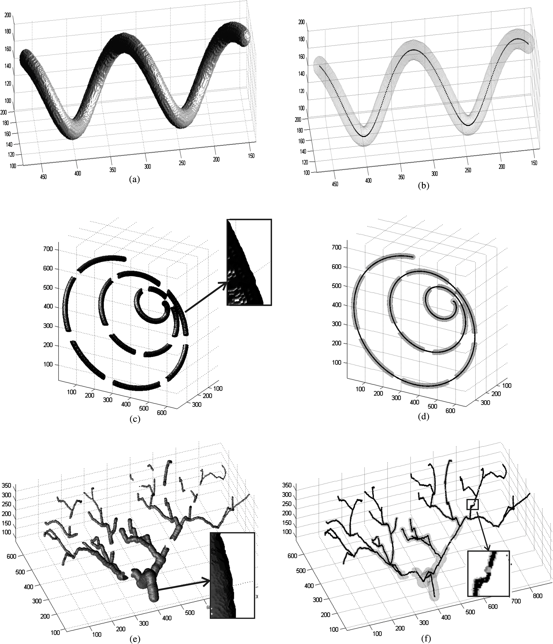 Fig. 11Left column: Synthetic objects with centerlines of fixed shape. Boundary noise was added randomly. Right column: The corresponding ground truth and computed centerlines. For each object, the overlapping points between the ground truth centerline and the computed one are shown in black, the points belonging to the ground truth centerline but not the computed one are shown in green, and the points belonging to the computed centerline but not the ground truth centerline are shown in red. (a) and (b) A helix structure. (c) and (d) A spiral structure. (e) and (f) A tree structure. A vessel tree shows the ability to detect bifurcations. The vessel branches are 1 mm in diameter. 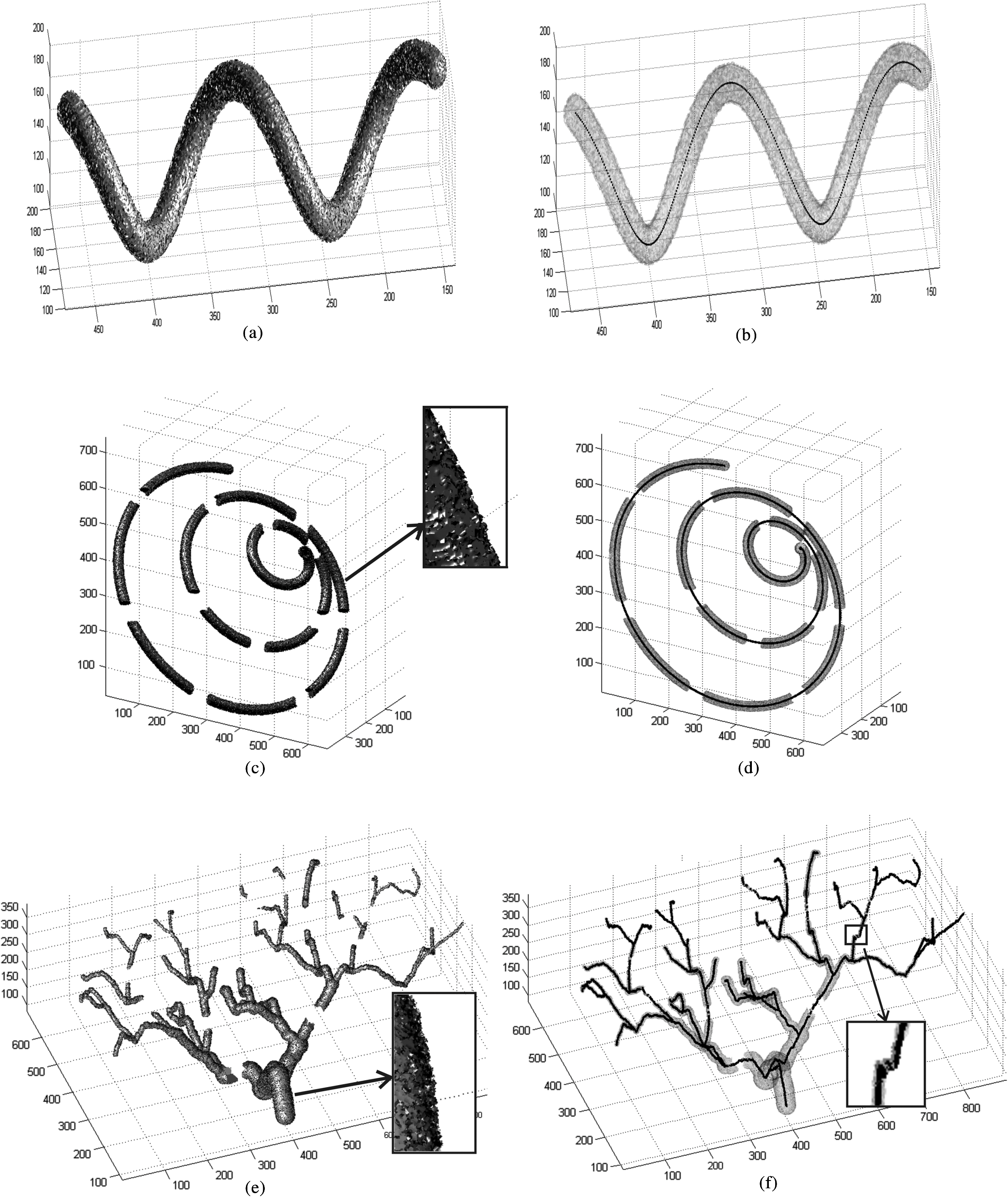 Table 1Validation of the centerline extraction algorithm for the synthetic objects.
The amount of overlap is consistently above 98% except for the noisy tree which has an overlap of 97.3%. The maximum distance is within 1.57 mm. However, the average distance is never more than 0.1 mm and in most cases is far less. These results provide some insight into how the method would behave for real medical data. First, the helix tube example shows that the method can handle structures with curvature. Second, the spiral phantom displays the ability of the approach to handle small vessel with small gaps. Third, the method can handle complex tree structures with small branches. Overall, our results provide quantitative evidence that the proposed algorithms perform well. 3.2.Extracting the Centerlines of Liver Artery from Abdominal CTIn liver surgery planning, the liver arteries play an important role in determining the optimal resections and in predicting blood supply to remaining liver tissue. The main problem in segmenting the liver arteries is that they are small and very poorly contrasted in the CT data, see Fig. 12. Another complicating factor is that the arteries run next to the larger portal veins, which increase the risk of segmentation leakage. Fig. 12Slices from the arterial phase of a CT angiography data set. The main problem in segmenting the liver arteries (arrows) is that they are small or very poorly contrasted in the CT data.  Eight abdominal CT angiography data sets were acquired using 64-row and dual-source CT scanners. The acquired image volumes are typically of the size with a pixel resolution of about and a slice thickness of 1.5 mm. The liver regions in the images were roughly hand-segmented by a radiology specialist and used as a mask. In our study, the manually marked center points of the vessels by two radiologists were used as the gold standard for quantitative evaluation of the extraction accuracy of the vessel centerline. The radiologists provided gold standards by manually tracking the vessel tree and marking the center of the vessels using a graphical user interface (GUI) developed in our laboratory. On the GUI, the sagittal view, axial view, and coronal view of the CT images corresponding to the region where a vessel is being tracked are displayed on a monitor. The GUI has functions allowing the user to cine-page through the CT slices, scroll in and out of individual vessels, adjust window setting, and zoom to improve visualization. The user can manually track the vessel trees by marking the vessel center points in any one of the three views at each vessel branch and the center point location will automatically propagate to all three views. Using the GUI, the radiologists marked the centerline for each branch, and labeled the anatomical level of the arteries. After marking center points of the arteries, the reconstruction of the discrete center points was performed using B-spline interpolation. In this section, a comparison is made with two state-of-the-art centerline detection methods. We briefly review the concept of both algorithms.
The vessel centerlines of the liver images included in the database were again segmented using the Wörz method, Agam method, and our method. Segmentation results of hepatic artery for three CT liver volumes are shown in Fig. 13. As shown in Fig. 13, the Wörz method and Agam method failed to extract small vessels in low contrast areas (rectangular regions). For the Wörz method, the tracking process terminated at the low contrast area, more seed points should be given for further process. Even when four seed points were given, the Wörz method still failed to extract the completed centerline in case 3. For the Agam method, the correlation-based filters can detect both small and large vessels due to the use of multiple sets of eigenvalues of the correlation matrix. However, the Agam method also failed for some small vessels. Averaged across all CT data sets, the overlap with the human expert extractions was used for accuracy evaluation. Accuracy results for the comparison are presented in Table 2. The results show that our method achieved the highest segmentation accuracy in comparison with these methods. Fig. 13Liver artery centerline segmented with three different methods. The first row, the second row and the third row illustrate the three different liver artery systems, respectively. First column shows the Wörz segmentation, the second column shows the Agam segmentation, and the third column shows our segmentation. In figure, the rectangular regions indicate several obvious failures; the black dots give the initial seed points for Wörz method; the blue lines show the centerlines of the manual segmentation; the red lines are the computed centerlines.  Table 2The overlap (%) between manual extraction and the computed extraction by three different methods on the eight liver artery data sets.
3.3.Extracting the Centerlines of Pulmonary Vessel from Chest CTMany of the published vessel segmentation and tracking methods provided accurate results in 2-D or 3-D images for vascular structures in the retina, brain, heart, etc. However, few studies have been conducted for segmentation, tracking, and reconstruction of the pulmonary vessel tree on CT images because the pulmonary vessels are more complicated compared to the vessels in other parts of the body in several aspects: widely distributed CT values, large variations of vessel sizes, and the complicated branching structures. We used three chest CT angiography data sets taken by 64-row and dual-source CT scanners. The volume size is with an in-slice pixel resolution of and slice thickness was 1.5 mm. In our vessel segmentation scheme, the lung region is first extracted to reduce computation time and avoid the effects caused by other nonvascular structures such as ribs, motion artifacts of the heart, and the edges of the heart and chest walls. An automatic segmentation method23 was applied to the volume of the scan within the patient body to extract lung regions. For the three clinical cases, there is no “ground truth” to prove the presence or absence of the vessels and their sizes. In our study, the manually marked center points of the vessels by three radiologists were used as the gold standard for quantitative evaluation of the segmentation accuracy of the vessels. A total of 2655, 2782, and 2853 vessel center points were marked by radiologists, respectively, for cases 1, 2, and 3. It is a demanding task for radiologists to mark the center points manually along small peripheral vessels on images displayed on a computer monitor. The radiologists decided to stop marking the center points on the peripheral vessels at certain levels, leaving some vessels not marked. Therefore, a visual inspection was performed to evaluate those vessels that were not marked by radiologists. Figure 14(b) shows an example of the manually marked vessel center points (red points) superimposed on the computer segmented vessel centerline. Figure 14(c) shows another view from the automatically segmented vessel centerlines shown in Fig. 14(b). It can be seen that many of the small vessels not marked by radiologists were extracted by our segmentation method. These small vessels were estimated to be smaller than 2 mm in diameter by manual measurement using an electronic ruler on the computer GUI. The accuracy of the vessel centerline segmentation was evaluated using three data sets. Averaged across three data sets, average distance to the ground-truth centerlines, was 0.32 mm. Fig. 14Comparison of radiologist’s marked vessel center points (gold standard vessel center points) with the automatically segmented vessel centerlines. To facilitate visualization, we give 700 marked vessel center points. (a) Slices of a chest CT angiography data set. (b) One view from the automatically segmented vessel centerlines within the left and right lungs superimposed with the gold standard vessel center points (red points). (c) Another view from the automatically segmented vessel centerlines within the left and right lungs superimposed with the gold standard vessel center points (red points). 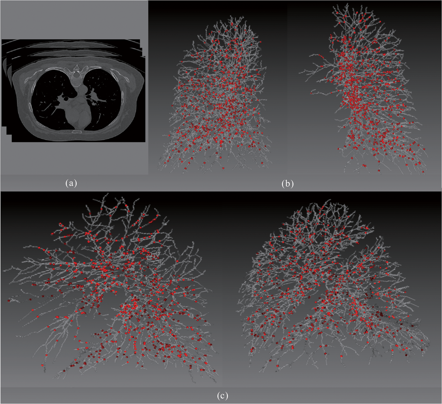 4.DiscussionsA fully automatic framework for vessel centerline extraction based on a multistep scheme has been presented. Our approach includes three major steps: (1) enhancing thin vessel, (2) extracting vessel centerline segment candidates, and (3) grouping and selecting vessel centerline segment. Not all of these steps are always required. For the thick vessels (in diameter ), vessel enhancement step may be omitted. This approach has five main advantages. First, compared to existing vessel centerline tracking approaches, it does not need user intervention; and an automatic vessel centerline extracting is performed by using a global optimization algorithm. Second, with a filter of 13 orientations, the approach can detect low-contrast and narrow vessel. Third, some methods often fail to connect segments belonging to one vessel in low contrast areas, our approach can fill gaps in blood vessels. Fourth, our framework avoids incomplete and disconnected extraction of the vessel centerline. And fifth, the approach is robust to noise and can produce vessel centerline extractions that have level of variability similar to those segmentations obtained from human raters. Quantitative evaluation of vessel centerline accuracy is a challenging problem because there is no ground truth for the vessel centerline extraction for clinical cases. Although a tubular phantom can be constructed with known vessels, it is difficult to construct a realistic phantom with a complete arterial tree mimicking complicated vascular structures. In a recent study by Shikata et al.24 about 2000 points were manually placed along the pulmonary vessels in each case as true vessel points for quantitative evaluation of a pulmonary vascular tree segmentation method. This method will provide an estimate of the fraction of the vessel tree segmented by the computer relative to that marked manually if the representative points are placed with reasonably balanced distribution in the entire pulmonary vascular tree. It is a demanding task for radiologists to mark the center points manually along small peripheral vessels on images displayed on a computer monitor. The radiologists decided to stop marking the center points on the peripheral vessels at certain levels, leaving some vessels not marked. Therefore, a visual inspection was performed to evaluate those vessels that were not marked by radiologists (Fig. 14). In our experiment using the chest CT data sets, three patient cases were used. Although the number of cases is small, the total number of center points that mark the entire pulmonary vessel tree down to very small vessels, for example, the segmental and sub segmental levels of arteries is quite large (more than 8290 for three cases). The evaluation including quantitative comparison and visual inspection on these three cases allows us to obtain a reasonable assessment of the vessel centerline extraction performance in this preliminary study. The computation time has also been considered, which might be critical in some applications. In the present study, the methods have been programmed using MATLAB 6.5 in an Intel(R) Core(TM) i5-4440 computer, 3.2 GHz, 16 G RAM. The processing time of the proposed method was about 8 min for one liver artery system and about 72 min for one chest CT angiography data. 5.ConclusionWe have successfully developed an automatic method for the 3-D vessel centerline extraction in CT images. Experimental results on synthetic and clinical data sets have shown that our method can extract complete and continuous centerline in the problematic regions that contain small and low-contrast vessels, and gaps between vessels. The extraction algorithm has high robustness toward noise and can produce vessel centerline extractions that have level of variability similar to those obtained manually. This study suggests that the proposed framework can be good enough to replace the time-consuming and tedious slice-by-slice manual extraction approach. In the future work, we plan to get a complete segmentation of the vessels. These structures need to be filled starting from the detected centerlines. AcknowledgmentsThe authors would like to thank the anonymous reviewers for constructive suggestions. This work is supported by the National Natural Science Foundation of China under Grant No. 61073124; the National Basic Research Program of China (973) under Grant 2011CB707701. ReferencesS. R. Fleagleet al.,
“Automated analysis of coronary arterial morphology in cineangiograms: geometric and physiological validation in humans,”
IEEE Trans. Med. Imaging, 8
(4), 387
–400
(1989). http://dx.doi.org/10.1109/42.41492 ITMID4 0278-0062 Google Scholar
J. H. C. Reiberet al.,
“Coronary artery dimensions from cineangiograms-methodology and validation of a computer-assisted analysis procedure,”
IEEE Trans. Med. Imaging, 3
(3), 131
–141
(1984). http://dx.doi.org/10.1109/TMI.1984.4307669 ITMID4 0278-0062 Google Scholar
Y. Satoet al.,
“A viewpoint determination system for stenosis diagnosis and quantification in coronary angiographic image acquisition,”
IEEE Trans. Med. Imaging, 17
(1), 121
–137
(1998). http://dx.doi.org/10.1109/42.668703 ITMID4 0278-0062 Google Scholar
J. H. C. ReiberP. W. SerruysJ. D. Barth,
“Quantitative coronary angiography,”
Cardiac Imaging, 211
–280 Philadelphia, Pennsylvania, Saunders(1991). Google Scholar
C. SeilerR. L. KirkeeideK. L. Gould,
“Basic structure-function relations of the epicardial coronary vascular tree,”
Circulation, 85
(6), 1987
–2003
(1992). CIRCAZ 0009-7322 Google Scholar
K. PalágyiA. Kuba,
“A parallel 3D 12-subiteration thinning algorithm,”
Graphical Models and Image Proc., 61
(4), 199
–221
(1999). http://dx.doi.org/10.1006/gmip.1999.0498 CGMPE5 1049-9652 Google Scholar
C. LohouG. Bertrand,
“Two symmetrical thinning algorithms for 3D binary images, based on P-simple points,”
Pattern Recogn., 40
(8), 2301
–2314
(2007). http://dx.doi.org/10.1016/j.patcog.2006.12.032 PTNRA8 0031-3203 Google Scholar
M. Dinget al.,
“An extension to 3D topological thinning method based on LUT for colon centerline extraction,”
Comput. Methods Programs Biomed., 94
(1), 39
–47
(2009). http://dx.doi.org/10.1016/j.cmpb.2008.10.002 CMPBEK 0169-2607 Google Scholar
A. Canet al.,
“Rapid automated tracing and feature extraction from retinal fundus images using direct exploratory algorithms,”
IEEE Trans. Inf. Technol. Biomed., 3
(2), 125
–138
(1999). http://dx.doi.org/10.1109/4233.767088 ITIBFX 1089-7771 Google Scholar
O. WinkW. J. NiessenM. A. Viergever,
“Fast delineation and visualization of vessels in 3-D angiographic images,”
IEEE Trans. Med. Imaging, 19
(4), 337
–346
(2000). http://dx.doi.org/10.1109/42.848184 ITMID4 0278-0062 Google Scholar
S. R. AylwardE. Bullitt,
“Initialization, noise, singularities, and scale in height ridge traversal for tubular object centerline extraction,”
IEEE Trans. Med. Imaging, 21
(2), 61
–75
(2002). http://dx.doi.org/10.1109/42.993126 ITMID4 0278-0062 Google Scholar
C. McIntoshG. Hamarneh,
“Vessel crawlers: 3D physically-based deformable organisms for vasculature segmentation and analysis,”
in Proc. IEEE Computer Society Conf. Computer Vision and Pattern Recognition,
1084
–1091
(2006). Google Scholar
M. VlachosE. Dermatas,
“Multi-scale retinal vessel segmentation using line tracking,”
Comput. Med. Imaging Graph., 34
(3), 213
–227
(2010). http://dx.doi.org/10.1016/j.compmedimag.2009.09.006 1063-6919 Google Scholar
A. A. Isolaet al.,
“Cardiac motion-corrected iterative cone-beam CT reconstruction using a semi-automatic minimum cost path-based coronary centerline extraction,”
Comput. Med. Imaging Graph., 36
(3), 215
–226
(2012). http://dx.doi.org/10.1016/j.compmedimag.2011.12.005 1063-6919 Google Scholar
R. ManniesingM. A. ViergeverW. J. Niessen,
“Vessel enhancing diffusion: a scale space representation of vessel structures,”
Med. Image Anal., 10
(6), 815
–825
(2006). http://dx.doi.org/10.1016/j.media.2006.06.003 MIAECY 1361-8415 Google Scholar
O. Frimanet al.,
“Multiple hypothesis template tracking of small 3D vessel structures,”
Med. Image Anal., 14
(2), 160
–171
(2010). http://dx.doi.org/10.1016/j.media.2009.12.003 MIAECY 1361-8415 Google Scholar
W. C. K. WongA. C. S. Chung,
“Probabilistic vessel axis tracing and its application to vessel segmentation with stream surfaces and minimum cost paths,”
Med. Image Anal., 11
(6), 567
–587
(2007). http://dx.doi.org/10.1016/j.media.2007.05.003 MIAECY 1361-8415 Google Scholar
Y. Satoet al.,
“Three-dimensional multi-scale line filter for segmentation and visualization of curvilinear structures in medical images,”
Med. Image Anal., 2
(2), 143
–168
(1998). http://dx.doi.org/10.1016/S1361-8415(98)80009-1 MIAECY 1361-8415 Google Scholar
S. FischerG. CristobalR. Redondo,
“Sparse overcomplete Gabor wavelet representation based on local competitions,”
IEEE Trans. Image Process., 15
(12), 3784
–3789
(2006). http://dx.doi.org/10.1109/TIP.2006.884913 IIPRE4 1057-7149 Google Scholar
K. Torkkola,
“Feature extraction by non-parametric mutual information maximization,”
J. Mach. Learn. Res., 3
(3), 1415
–1438
(2003). 1532-4435 Google Scholar
S. WörzK. Rohr,
“3D adaptive model-based segmentation of human vessels,”
Proc. SPIE, 6511 65110Q
(2007). http://dx.doi.org/10.1117/12.709286 PSISDG 0277-786X Google Scholar
G. AgamS. G. Armato IIIC. Wu,
“Vessel tree reconstruction in thoracic CT scans with application to nodule detection,”
IEEE Trans. Med. Imaging, 24
(4), 486
–99
(2005). http://dx.doi.org/10.1109/TMI.2005.844167 ITMID4 0278-0062 Google Scholar
S. HuE. A. HoffmanJ. M. Reinhardt,
“Automatic lung segmentation for accurate quantitation of volumetric X-ray CT images,”
IEEE Trans. Med. Imaging, 20
(6), 490
–498
(2001). http://dx.doi.org/10.1109/42.929615 ITMID4 0278-0062 Google Scholar
H. ShikataE. A. HoffmanM. Sonka,
“Automated segmentation of pulmonary vascular tree from 3D CT images,”
Proc. SPIE, 5369 107
–116
(2004). http://dx.doi.org/10.1117/12.537032 PSISDG 0277-786X Google Scholar
BiographyYuanzhi Cheng received his PhD degree from Osaka University, Osaka, Japan, in 2007. He is currently an associate professor in the School of Computer Science and Technology, Harbin Institute of Technology. He has published more than 30 papers in scientific journals. His research interests are concentrated on pattern recognition, medical image processing, and computer-assisted surgical system. Yadong Wang is currently a professor in the School of Computer Science and Technology, Harbin Institute of Technology. His research interests include pattern recognition, machine learning and bioinformatics. He has published more than 60 papers in scientific journals. Shinichi Tamura received his PhD degrees in electrical engineering from Osaka University, Osaka, Japan, in 1971. He is currently a professor in the Center for Advanced Medical Engineering and Informatics, Osaka University. He has published more than 260 papers in scientific journals and received several awards from journals, including Pattern Recognition and Investigative Radiology. His current research activities include works in the field of medical image analysis and its applications. He is a fellow of IEEE. |
||||||||||||||||||||||||||||||||||||||||||||||||||||||||||||||||||||||||