Image fusion with nonsubsampled contourlet transform and sparse representation

Jun Wang; Jinye Peng; Xiaoyi Feng; Guiqing He; Jun Wu; Kun Yan

doi:10.1117/1.JEI.22.4.043019

19 November 2013 Image fusion with nonsubsampled contourlet transform and sparse representation

Jun Wang, Jinye Peng, Xiaoyi Feng, Guiqing He, Jun Wu, Kun Yan

Author Affiliations +

Journal of Electronic Imaging, Vol. 22, Issue 4, 043019 (November 2013). https://doi.org/10.1117/1.JEI.22.4.043019

Abstract

Image fusion combines several images of the same scene into a fused image, which contains all important information. Multiscale transform and sparse representation can solve this problem effectively. However, due to the limited number of dictionary atoms, it is difficult to provide an accurate description for image details in the sparse representation–based image fusion method, and it needs a great deal of calculations. In addition, for the multiscale transform–based method, the low-pass subband coefficients are so hard to represent sparsely that they cannot extract significant features from images. In this paper, a nonsubsampled contourlet transform (NSCT) and sparse representation–based image fusion method (NSCTSR) is proposed. NSCT is used to perform a multiscale decomposition of source images to express the details of images, and we present a dictionary learning scheme in NSCT domain, based on which we can represent low-frequency information of the image sparsely in order to extract the salient features of images. Furthermore, it can reduce the calculation cost of the fusion algorithm with sparse representation by the way of nonoverlapping blocking. The experimental results show that the proposed method outperforms both the fusion method based on single sparse representation and multiscale decompositon.

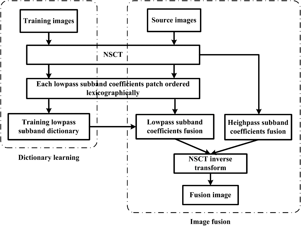
1. Introduction

Image fusion is a process of combining several source images that are captured by multiple sensors or by a single sensor at different times. Those source images contain more comprehensive and accurate information than a single image. Image fusion is widely used in the field of military, medical imaging, remote sensing imaging, machine vision, and security surveillance.¹^,²

In recent decades, many fusion algorithms have been proposed. Most of these methods can be classified into two categories: multiscale transform and sparse representation–based approach. The basic idea of multiscale transform–based fusion method is that the salient information of images is closely related to the multiscale decomposition coefficient. These methods usually consist of three steps, including decomposing source image into multiscale coefficients, fusing these coefficients with a certain rule, and reconstructing a fused image with inverse transformation. Multiscale transform-based fusion methods include the gradient pyramid,³ Laplacian pyramid,⁴ discrete wavelet transform (DWT),⁵ stationary wavelet transform (SWT),⁶ and nonsubsampled contourlet transform (NSCT).⁷ Image fusion by these methods is a multiscale approach for image representation and has fast implementation.

Image fusion with sparse representation method is based on the idea that image signals can be represented as a linear combination of a “few” atoms from learned dictionary, and the sparse coefficients are treated as the salient features of the source images. The main steps include (1) dictionary learning, (2) sparse representation of the source image, (3) fusion of this sparse representation by the fusion rule, (4) reconstruction of the fused image. Among them, steps (1) and (3) are the most critical factors in successful fusion. The fusion results among overcomplete discrete cosine transform (DCT) dictionary, the hybrid dictionary, and the trained dictionary are compared and studied in Refs. 8 and 9. The fusion results demonstrate that the trained method provides the best performances. Fusion rules of sparse representation–based methods are researched in Refs. 10 and 11. The former one pursues the sparse vector for the fused image by optimizing the Euclidean distances between fused image and source image. The latter one represents source image with the common and innovation sparse coefficients and combines them by the mean absolute values of the innovation coefficients. In Ref. 12, steps (1) and (3) are both studied. During dictionary learning stage, it is implemented by joint sparse coding and singular value decomposition (SVD). And for the new fusion rule, it combines the weighted average with the choose-max rule.

Both of the above fusion methods have their special advantages as well as some disadvantages. The multiscale transform–based methods are multiscale approaches for image representation and have fast implementation. However, the sparsity of coefficients that represent the image could be increased significantly in the low-pass subbands, where approximate zero coefficients are very few, i.e., they are unable to express low-frequency information of images sparsely, while sparse representation can effectively extract the underlying information of source images.⁹ If low-frequency coefficients are integrated directly, it will degrade the performance of the fused result because the low-frequency coefficients contain the main energy of the image.

In contrast, the second method allows for more meaningful representations from source images by learned dictionary, which are more finely fitted to the data,¹³ thus producing better performance. However, due to the limited number of atoms in a dictionary, it is difficult to provide the accurate representation of image details, such as edges and textures. Moreover, complexity constraints the atom size in the learned dictionary (a typical size is of the order of 64)¹⁴. This limitation is the reason why patch-based processing is so often practiced when using such dictionaries. To avoid blocking-artifact, the step size usually is 1.⁸^–¹³ However, along with the increase of image size, the number of image blocks grows exponentially, and a great deal of calculation is needed.

In this paper, we attempt to merge the advantages of the above two methods. An NSCT and sparse representation–based image fusion method is proposed, namely NSCTSR. We decompose the source images by NSCT to obtain the near sparseness of high-pass subband at multiscale and multidirection to represent image details. For the problem of nonsparseness of low-frequency subband in the NSCT domain, we train the dictionary for the low-pass coefficients of the NSCT to obtain more sparse and salient feature of source images in NSCT domain. Then the low-pass and high-pass subbands are integrated according to different fusion rules, respectively. Moreover, the proposed method can reduce the calculation cost by nonoverlapping blocking.

The rest of the paper is organized as follows: Sec. 2 reviews the theory of the NSCT in brief. Section 3 presents dictionary learning in NSCT domain. In Sec. 4, we propose the fusion scheme, whereas Sec. 5 contains experimental results obtained by using the proposed method and a comparison with the state-of-the-art methods. Section 6 concludes this paper.

2. Nonsubsampled Contourlet Transform

NSCT is proposed on the grounds of contourlet conception, which discards the sampling step during the image decomposition and reconstruction stages.¹⁵ Furthermore, NSCT presents the features of shift-invariance, multiresolution, and multidimensionality for image presentation by using a nonsampled filter bank iteratively. When the NSCT is introduced to image fusion, more information for fusion can be obtained and the impacts of misregistration on the fused results can also be reduced effectively. Therefore, the NSCT is more suitable for image fusion.¹⁶

The structure of NSCT consists of two parts: nonsubsampled pyramid (NSP) and nonsubsampled directional filter banks (NSDFB).¹⁷ First, image is decomposed by NSP with different scales to obtain subband coefficients at different scales. And then those coefficients are decomposed by NSDFB and thereby subband coefficients are obtained at different scales and different directions. Figure 1 shows NSCT.

Fig. 1

Nonsubsampled contourlet transform (NSCT).

In NSCT, the multiscale property is accomplished by using two-channel nonsubsampled two-dimensional filter banks, which can achieve a subband decomposition similar to Laplacian pyramid. Figure 2 shows the NSP decomposition with $J = 3$ . Such expansion is conceptually similar to the one-dimensional nonsubsampled wavelet transform, which is applied in the à trous algorithm.¹⁷ The directional filter bank in NSCT is constructed by combining critically sampled two-channel fan filter banks and resampling operations as $H_{0} (Z)$ and $H_{1} (Z)$ shown in Fig. 2. A shift-invariant directional expansion is obtained with an NSDFB, which is constructed by eliminating the downsamplers and upsamplers in the DFB.¹⁸ Figure 3 illustrates the four-channel decomposition. There is a low-pass subband and $\sum_{j = 0}^{J - 1} 2^{l_{j}}$ high-pass subband when image is decomposed by NSCT decomposition, where $l_{j}$ denotes the number of levels in the NSDFB at the $j$ ’th scale.

Fig. 2

Three-stage pyramid decomposition directional.

Fig. 3

Four-channel nonsubsampled filter bank constructed with two-channel fan filter banks.

3. Sparse Representation in NSCT Domain

3.1.

Sparse Representation for Image Fusion

Sparse representation is based on the assumption that a signal can be expressed as a sparse combination of atoms from dictionary. Formally, for a signal $y \in R^{n \times 1}$ , its sparse representation is solved by the following optimization problem:

Eq. (1)

\min_{x} {‖ x ‖}_{0}^{0} s.t {‖ y - D x ‖}_{2} \leq ϵ,

where

D \in R^{n \times K}

is a dictionary that contains the atoms as its columns,

x \in R^{K \times 1}

is a vector, the expression

{‖ α ‖}_{0}^{0}

is a count of the number of nonzeroes in the vector

α

, and

ε

is error tolerance. The process of solving the above optimization problem is commonly referred to as sparse-coding.

Theoretically, the sparse representation globally expresses an image, but it cannot directly deal with image fusion. On one hand, computational complexity limits the atom size that can be learned;¹⁹ on the other hand, image fusion depends on the local information of source images. Thus, patch-based processing is adopted to make the sparse representation.²⁰ A sliding window is used to divide source image, from left-top to right-bottom, into patches. Then, these patches are transformed into vectors via lexicographic ordering.

3.2.

Dictionary Learning with K-SVD in NSCT Domain

One of the fundamental questions in sparse representation model is the choice of dictionary. The K-SVD algorithm has been widely used to obtain such dictionary via approximating the following problem:²¹

Eq. (2)

\underset{D, X}{\arg \min} {‖ Y - DX ‖}_{F}^{2} s.t. {‖ x_{i} ‖}_{0}^{0} \leq T \forall i,

where

Y = [y_{1} y_{2} \dots y_{N}] \in R^{n \times N}

denotes the set of training examples,

X \in R^{K \times N}

is the sparse coefficient matrix (

x_{i}

are the columns of

X

), and

T

stands for sparsity.

Based on the theory above, we should learn a low-pass overcomplete dictionary $D_{l}$ in order to sparsely represent images in NSCT domain. We begin our derivation by the following modification of Eq. (2):

Eq. (3)

\underset{D, X}{\arg \min} {‖ C_{S} - DX ‖}_{F}^{2} s.t. {‖ x_{i} ‖}_{0}^{0} \leq T \forall i .

Here, we decompose the training image $I$ by NSCT. Assuming that $W_{S}$ is the NSCT analysis operator, $W_{S} I = C_{S}$ , and $C_{S}$ is the decomposition coefficient of NSCT.

Substituting $W_{S} I = C_{S}$ into Eq. (3), we can equivalently write

Eq. (4)

\underset{D, X}{\arg \min} {‖ W_{s} I - DX ‖}_{F}^{2} s.t. {‖ x_{i} ‖}_{0}^{0} \leq T \forall i .

The above formulation suggests that we can learn our dictionary in the analysis domain. A natural way to view the NSCT analysis domain is not as a single vector of coefficients, but rather as a collection of coefficient images or bands. Consider that the different subband images of NSCT contain information at different scales and orientations. We achieve this by training subdictionaries separately for each band.

Eq. (5)

\forall b, \underset{D_{b}, X_{b}}{argmin} {‖ {(W_{S} I)}_{b} - D_{b} X_{b} ‖}_{F}^{2} s.t. {‖ x_{i, b} ‖}_{0}^{0} \leq T \forall i,

where subscript

b = 1, 2, \dots, B

denotes the different NSCT coefficient bands and

B

is the total number of subband. However, the distribution of NSCT subband coefficients is that the low-pass subband coefficients have large amplitude and contain more information, whereas high-pass coefficients have small amplitude, usually fluctuate around 0, contain less information, and are likely to produce overfitting.²² Therefore, in this paper, we learn dictionary in low-frequency subband only and the complete learning algorithm is described as follows:

1. Decompose each of the training-set images using NSCT and extract one low-pass and $B - 1$ high-pass subbands;
2. Set the dictionary matrices to initial the low-pass dictionary $D_{l} \in R^{n \times K}$ ;
3. Extract maximally overlapping patches of size $\sqrt{n} \times \sqrt{n}$ from the low-pass band $L_{k} {k = 1, 2, \dots, K}$ of all training images, and each patch is ordered lexicographically as vector. Then, all the vectors in image $L_{k}$ are constituted into one matrix $V_{k}$ and $\underset{̲}{V} = [V_{1} V_{2} \dots V_{K}]$ ;
4. The overcomplete dictionary $D_{l}$ is trained by solving the following approximation problem:
Eq. (6)
$\underset{D_{l} {, X}_{b}}{argmin} {‖ \underset{̲}{V} - D_{l} X_{l} ‖}_{F}^{2} s.t. {‖ x_{i, l} ‖}_{0}^{0} \leq T \forall i .$
The above procedure is shown in Fig. 4.

Fig. 4

Dictionary learning in low-pass sub-band of NSCT.

4. Proposed Image Fusion Scheme

Low-frequency information of images are reflected by the low-frequency subband, which includes the main image energy. If we integrate them directly, the important information is not easy to extract due to the low sparsity of the low-pass subband, whereas high-frequency information of images are sparse approximately. Consequently, we will design different rules for these subbands.

4.1.

Low-Pass Subband Coefficients Fusion

The sparse vector of low-pass subband can be obtained by solving the following problem with $D_{l}$ , which was trained in Sec. 3.2:

Eq. (7)

\min_{x} ‖ x_{i, l} ‖_{0}^{0} s.t. {‖ \underset{̲}{V} - D_{l} X_{l} ‖}_{F}^{2} \leq ϵ,

where

\underset{̲}{V}

is composed of the low-pass subband of NSCT decomposition of source images. The above optimization problem is generally nondeterministic polynomial (NP)-hard; approximate solutions can be found. In this paper, we use orthogonal matching pursuit (OMP) to obtain the sparse representation due to its simplicity and fast execution.

Then, the activity level of the $i$ ’th block in low-pass subband is ${‖ x_{i, l} ‖}_{1}$ , which represents salient features of an image. The purpose of image fusion is to transform all the important information from input source images into fused image, so we use the following fusion rule:

1. By sliding window technique, each low-pass subband coefficient of source image $L_{k}$ is divided into $\sqrt{n} \times \sqrt{n}$ patches with $step \in [1, \sqrt{n}]$ . Then, all the patches are transformed into vectors via lexicographic ordering and ${V_{i}^{k}}_{i = 1}^{[(M - \sqrt{n}) / step + 1] [(N - \sqrt{n}) / step + 1]}$ are obtained.
2. Sparsely represent the vectors at each position, $i$ , with different $V_{i}^{k}$ , using OMP and obtain ${x_{i, l}^{1}, x_{i, l}^{2}, \dots, x_{i, l}^{K}}$ .
3. Combine the sparse coefficient vectors using the max-activity level rule.
Eq. (8)
$x_{i, l}^{f} = x_{k^{*}, l}, k^{*} = \underset{k = 1, 2, \dots, K}{\arg \max} ({‖ x_{i, l}^{k} ‖}_{1}) .$
4. Steps 2 and 3 are applied to all the subband blocks. Thus, we can get ensemble of all fused coefficients $X_{l}^{F} = {x_{i, l}^{f}}_{i = 1}^{[(M - \sqrt{n}) / step + 1] [(N - \sqrt{n}) / step + 1]}$ . Then, the vector of low-pass subband of the fused image can be calculated by $V_{l}^{F} = D_{l} \times X_{l}^{F}$ , where $V_{l}^{F} \in R^{n \times {[(M - \sqrt{n}) / step + 1] [(N - \sqrt{n}) / step + 1]}}$ .
5. The low-pass subband of fused image $L^{F}$ is reconstructed using $V_{l}^{F}$ . Each vector $v_{i, l}^{F}$ in $V_{l}^{F}$ is reshaped into a block of size $\sqrt{n} \times \sqrt{n}$ ; then the block is added to $L^{F}$ at its responding position. Thus, for each pixel position, the pixel value is the sum of several block values, which is divided by the adding times at its position to obtain the final reconstructed result.

4.2.

High-Pass Subband Coefficients Fusion

NSCT not only provides multiscale analysis for images, but also captures minutiae features, such as the edge, linear features, and regional boundaries in high-pass subband of source images. We find out that there are several characteristics in the high-frequency coefficients: first, near sparsity. The detail components of the source image are usually expressed in all directions of same scale with large values, while the values of nondetails of images are practically nil. Second, the larger the absolute value of the subband coefficients is, the more edges and texture information it contains. The coefficients of an image are meaningful to emphasize and detect salient features. Besides, we notice that the strong edges have large coefficients on the same scale in all directions. Considering above factors, high-pass subband coefficients are integrated by the following steps:

The information of source images in the directional subbands with $2^{- l}$ scale is defined by

Eq. (9)

H_{l} (n, m) = \sum_{1 \leq h \leq g_{l}} | H_{l, h} (n, m) | .

Fuse the high-pass subband coefficients to generate $H_{l, h}^{F} (n, m)$ according to their information of directional subbands. The fused coefficients of $2^{- l}$ scale in $(n, m)$ pixel position is obtained as

Eq. (10)

H_{l, h}^{F} (n, m) = H_{l, h}^{k^{*}} (n, m), k^{*} = \underset{k = 1, \dots, K}{\arg \max} | H_{l} (n, m) |,

where

0 \leq l \leq J - 1, 1 \leq h \leq g_{l}

, and

g_{l}

denotes the number of high-pass subband coefficients in the

2^{- l}

scale.

4.3.

Fusion Scheme

The proposed image fusion method is illustrated in Fig. 5, and the whole fusion scheme is as follows:

1. Dictionary learning in NSCT domain in accordance with Sec. 3.2 and low-frequency dictionary $D_{l}$ is obtained.
2. Decompose the source images into one low-pass subband and a series of high-pass subbands, respectively.
3. Fuse low-pass subband by the process described in Sec. 4.1 with trained dictionary in step 1 and obtain the low-pass subband coefficients of fused image $L^{F}$ .
4. Select fusion NSCT coefficients for each high-pass subband from source images according to Sec. 4.2, that is $H_{l, h}^{F}, (l \in [1, J], h \in [1, g_{l}])$ .
5. Reconstruct the fused image $I^{F}$ based on the $L^{F}$ and $H_{l, h}^{F}, (l \in [1, J], h \in [1, g_{l}])$ by taking an inverse NSCT transform.

Fig. 5

Procedure of image fusion based NSCT and sparse representation.

5. Experiments

In this section, the proposed fusion algorithm is compared with four multiscale transform–based methods, including DWT, SWT, NSCT,⁷ and LPSSIM [LPSSIM is an image fusion method proposed by Ref. 4, which fuses Laplacian Pyramid coefficients of source images by using structural similarity metric (SSIM). So we abbreviate it as LPSSIM for simplicity], and four sparse representation-based methods, i.e., SR⁸ (tradition sparse representation), simultaneous orthogonal matching pursuit (SOMP),⁹ joint sparse representation (JSR),¹¹ and method of optimal directions for joint sparse representation (MODJSR)-based fusion algorithms.¹² The parameters for different methods and evaluation metrics are first presented. Second, the performance of the NSCTSR-based method is demonstrated in comparison with the eight fusion algorithms. Then, in order to reduce the calculation amount of sparse representation–based methods, the sliding step with sliding window is also discussed. Finally, an experiment on larger image sets is presented to demonstrate the universality of the proposed method.

5.1.

Experimental Setup

In this experiment, for DWT- and SWT-based methods, the most popular setting, the max-abs fusion rule, is selected, and the wavelet basis is “db4” with three levels decomposition. We use “9-7” and “c-d” as the pyramid filter and the directional filter for NSCT,⁷ and the decomposition level is set to ${2^{2}, 2^{2}, 2^{3}, 2^{4}}$ , all these parameters same as the proposed based method. The parameter $α = 1$ , and LP decomposition is three in LPSSIM-based method. For the four sparse representation–based methods, the training set for the learned dictionary is constructed by 100,000 patches randomly selected from 50 images in Image Fusion Server;²³ the patch size and dictionary size are set as $8 \times 8$ and $64 \times 256$ , which are widely used in image fusion methods.⁸^–¹² We set the error tolerance $ε = 0.001$ at sparse coding and sparsity $T = 10$ at dictionary learning.

We use five evaluation criteria: local importance quality index $Q_{0}$ ,²⁴ weighted fusion quality index $Q_{W}$ ,²⁵ edge-dependent fusion quality index $Q_{E}$ ,²⁵ local similarity quality index $Q_{G}$ ⁴ and $Q_{A B / F}$ ,²⁶ which evaluates the fusion algorithm in transferring input gradient information into the fusion result. All of these should be as close to 1 as possible. All the experiments are completed in the environment of a Pentium dual-core CPU 2.79 GHz PC with 2-GB RAM, operating under MATLAB R2012b.

5.2.

Fusion Results

Image fusion experiments were carried out on different images. Figure 6 depicts a pair of medical images; the left image is computed tomography (CT) image, and the right one is magnetic resonance imaging (MRI) image. The CT image shows structures of bone, while the MRI image shows the areas of soft tissue details. Figure 7 shows the fused images by various tested methods, and the local amplification of these results is shown in Fig. 8 for easy observation. Figures 7(a) and 8(a) reveal that the DWT-based method produces more artificial images. From the right image in each set of Fig. 8, we can see that, motivated by the multiscale transform, the SWT-, NSCT-, and LPSSIM-based methods reserve the details more completely than SR-, SOMP-, and JSR-based methods. However, from the left side, it can be seen that SR-, SOMP-, and JSR-based methods have much clearer skeletal features than SWT, NSCT, and LPSSIM fused images, due to the sparse representation, which can extract the salient features of source images. What is more, the NSCTSR fused image exhibits better visual quality with much clearer soft tissues and bone structures than compared methods. Second is the method of optimal directions for joint sparse representation-based image fusion (MODJSR) fused image, which loses only some soft tissue details as can be seen in the left image in Fig. 8(h), while the details are also important for diagnosing. Table 1 reports the objective evaluation of various methods and the best results are indicated in bold. We can see that the NSCTSR-based method achieved the best results in four of the five evaluation metrics, i.e., $Q_{0}$ , $Q_{W}$ , $Q_{A B / F}$ , $Q_{G}$ . As for $Q_{E}$ , the MODJSR method performed slightly better than our method.

Fig. 6

Original medical source images.

Fig. 7

Medical image fusion results using (a) discrete wavelet transform (DWT), (b) stationary wavelet transform (SWT), (c) NSCT, (d) LPSSIM, (e) SR, (f) SOMP, (g) JSR, (h) MODJSR, and (i)NSCTSR.

Fig. 8

Local amplification of (a) DWT, (b) SWT, (c) NSCT, (d) LPSSIM, (e) SR, (f) SOMP, (g) JSR, (h) MODJSR, and (i) NSCTSR.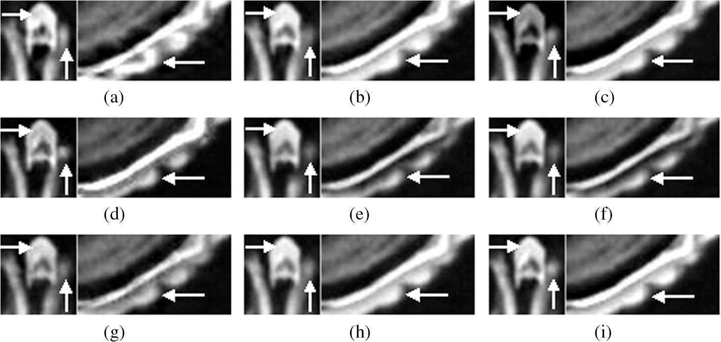

Table 1

The objective evaluation of various methods for medical images.

Methods	$Q_{0}$	$Q_{W}$	$Q_{E}$	$Q_{A B / F}$	$Q_{G}$
DWT	0.5674	0.6933	0.4301	0.637	0.7198
SWT	0.6257	0.7943	0.5159	0.7043	0.7557
NSCT	0.6256	0.7701	0.5368	0.6861	0.7691
LPSSIM	0.6352	0.8104	0.5565	0.6996	0.8141
SR	0.6526	0.7829	0.5469	0.7255	0.8004
SOMP	0.6676	0.7953	0.5486	0.7379	0.8140
JSR	0.6043	0.7784	0.5128	0.6667	0.7662
MODJSR	0.6681	0.8110	0.5606	0.7247	0.8117
NSCTSR	0.6896	0.8209	0.5598	0.7298	0.8247

Note: DWT, discrete wavelet transform; SWT, stationary wavelet transform; NSCT, nonsubsampled contourlet transform.

A pair of multisensor images is considered. The left image in Fig. 9 shows buildings and the right one provides roads and chimney more salient and obviously. Different fusion methods are shown in Fig. 10; the local amplification of these results are in Fig. 11, in which it will be convenient to observe roofs, roads, lanes, chimney, and the contrast of fused images. Careful inspection of Figs. 10(a) and 11(a) shows that the DWT fused image has Gibbs effect in some degree. In Figs. 10(b) to 10(i) and 11(b) to 11(i), it can be seen that the NSCTSR fused images have better contrast than NSCT fused images, are more smooth than SWT and LPSSM fused images, and, furthermore, have more clearer lanes and edges of chimney than SR, SOMP, JSR, and MODJSR fused images. Intuitively, more detailed information and significant features of the source images are transferred into the fused image by NSCTSR-based method than others. To evaluate this visual inspection objectively, the values of five evaluation criteria are listed in Table 2. Obviously, our proposed method is superior to others for all five criteria, which is consistent with the results of subjective evaluation.

Fig. 9

Original “input094” multisensor source images.

Fig. 10

The “input094” multisensor source image fusion results using (a) DWT, (b) SWT, (c) NSCT, (d) LPSSIM, (e) SR, (f) SOMP, (g) JSR, (h) MODJSR, and (i) NSCTSR.

Fig. 11

Local amplification of (a) DWT, (b) SWT, (c) NSCT, (d) LPSSIM, (e) SR, (f) SOMP, (g) JSR, (h) MODJSR, and (i) NSCTSR.

Table 2

The objective evaluation of various methods for “input094” multisensor images.

Methods	$Q_{0}$	$Q_{W}$	$Q_{E}$	$Q_{A B / F}$	$Q_{G}$
DWT	0.5742	0.7236	0.462	0.5155	0.7696
SWT	0.6370	0.7733	0.5303	0.5654	0.7940
NSCT	0.6546	0.7853	0.5621	0.5958	0.8189
LPSSIM	0.6647	0.7838	0.5723	0.6067	0.7800
SR	0.6568	0.7888	0.5701	0.6007	0.8208
SOMP	0.6528	0.7923	0.5703	0.6059	0.8245
JSR	0.6432	0.7715	0.5442	0.5883	0.7969
MODJSR	0.6700	0.7967	0.5625	0.5962	0.8250
NSCTSR	0.6707	0.7975	0.5739	0.6067	0.8279

Note: The bold values are the best results of individual evaluation criteria.

Analyzing the above results of subjective visual evaluation and objective indicators, we can see that the NSCTSR indicates image details more effectively than the sparse representation–based fusion method. The reason is the NSCT can extract high-frequency details of source images in multiscale and multidirectional ways. At the same time, compared with the multiscale transform–based image fusion, the NSCTSR can also extract the salient features of source images more sparsely and effectively. Consequently, the NSCTSR has better fusion performance.

5.3.

Discussion on the Sliding Step

As already mentioned in Sec. 3.2, the fusion methods based on sparse representation with trained dictionary are all accomplished by sliding window scheme. In order to avoid blocking artifacts, the sliding step is set as 1. If the size of the source image is $256 \times 256$ and the block is $8 \times 8$ as usual, the patches for each source image is 62,001. Sparse coding for all of these patches is time-consuming.⁹^,²⁰ In the same way, when the input image is $512 \times 512$ , the block number is 255,025. If the step value is increased, the number of blocks can be reduced dramatically, thus increasing the speed. For instance, by tiling the nonoverlapping blocks, the step is 8, the number of patches is 1,024 for image of $256 \times 256$ and 4,096 for image of $512 \times 512$ , and the calculation cost of nonoverlapping is only $\sim 1 / 60$ of the max-overlapping methods. Therefore, we discuss the sliding step with several sparse representation methods in this section.

The images are fused by DWT-, SWT-, NSCT-, and LPSSIM-based fusion methods and do not need sliding technology, and the results of SR, SOMP, JSR, MODJSR, and the NSCTSR-based method with moving $step = 1, 2, 4, 8$ are compared. Figures 12(c) to 12(k) show the fused outputs using the eight methods and the proposed method. It can be seen that the NSCTSR method has much better visibility than other methods whether on the overall visual effect of the image or image fine details (the building edge), which is consistent with previous section. Due to limited space, Figs. 12(l) to 12(p) exhibit only the effects of several sparse representation–based fusion methods with nonoverlapping, i.e., sliding step is 8, signed as NSCTSR_S8. From the figures, it is clear that fused results with SR-, SOMP-, JSR-, and MODJSR-based methods have obvious blocking artifacts, while the proposed method performs no blocking effect visually, which is because the fused image is reconstructed by NSCT inverse transform and the low-pass subband block effect has been progressively weakened.

Fig. 12

Fused images of several fusion algorithms and with the nonoverlapping block method. (a) and (b) Multisensor images. (c) DWT. (d) SWT. (e) NSCT. (f) LPSSIM. (g) SR. (h) SOMP. (i) JSR. (j). MODJSR. (k) NSCTSR. (l) SR_S8. (m) SOMP_S8. (n) JSR_S8. (o) MODJSR_S8. (p) NSCTSR_S8.

From the objective evaluation of analysis in Table 3, the two top results are indicated in bold. We conclude that single methods based on sparse representation are usually better than the single transform methods based on multiscale, but the former methods perform best with the smallest moving step, which needs large calculation. The quantitative assessments of the proposed method are almost constant with the distinct window, which is more effective than traditional sparse representation–based methods.

Table 3

The objective evaluation of various methods and some methods with the nonoverlapping block method. Two top results are indicated in bold.

Methods	$Q_{0}$	$Q_{W}$	$Q_{E}$	$Q_{A B / F}$	$Q_{G}$
DWT	0.6319	0.7300	0.4915	0.5323	0.7431
SWT	0.6797	0.7623	0.5488	0.5838	0.7740
NSCT	0.6915	0.7958	0.5977	0.6119	0.8152
LPSSIM	0.6691	0.7903	0.585	0.6231	0.8032
SR	0.7098	0.7961	0.6092	0.6112	0.7933
SOMP	0.7049	0.7927	0.6047	0.6297	0.7941
JSR	0.6861	0.7683	0.5538	0.5937	0.7629
MODJSR	0.6915	0.7746	0.5475	0.6034	0.8073
NSCTSR	0.7121	0.8079	0.6119	0.6373	0.8192
SR_S8	0.6818	0.7878	0.5817	0.5771	0.7839
SOMP_S8	0.6752	0.7649	0.5541	0.5948	0.7702
JSR_S8	0.5429	0.5889	0.233	0.4143	0.6003
MODJSR_S8	0.5526	0.609097	0.2449	0.4089	0.6209
NSCTSR_S8	0.7119	0.8078	0.6117	0.6371	0.8091

The quantitative assessments of several fusion methods with different sliding steps are shown in Fig. 13. We can see that the quantitative assessments of JSR and MODJSR are most affected by sliding step, which is followed by SOMP and SR; the proposed method is almost unaffected and has the best fusion result in terms of evaluation criteria including $Q_{0}$ , $Q_{W}$ , $Q_{E}$ , and $Q_{A B / F}$ . As for $Q_{G}$ , the NSCT-based method is somewhat better than NSCTSR_8.

Fig. 13

Fusion performance of several fusion methods with different sliding step. (a) $Q_{0}$ . (b) $Q_{W}$ . (c) $Q_{E}$ . (d) $Q_{A B / F}$ . (e) $Q_{G}$ _.

Similar observations are noted for the test case in Fig. 14. In this case, NSCTSR and NSCTSR_S8 are again able to provide the most visually pleasing fusion results. In Figs. 14(g) to 14(i), we can see that it is difficult for the single traditional fusion method based on sparse representation to reserve fusion detail features. The multiscale transform image fusion result in Figs. 14(c) to 14(f) has reduced contrast; it is useless without effective salient features. The fused image by NSCTSR can reserve the details and lines completely, and also highlight the significant information [Fig. 14(a) is bright and Fig. 14(b) is dark]. In the nonoverlapping block versions in Figs. 14(l) to 14(p), we also find that the proposed method is less affected by the block step than other sparse representation methods. From Table 4, it can be seen that the proposed method is still best on comprehensive comparison.

Fig. 14

Fused images of several fusion algorithms and with the nonoverlapping block method. (a) and (b) Navigation source images. (c) DWT. (d) SWT. (e) NSCT. (f) LPSSIM. (g) SR. (h) SOMP. (i) JSR. (j) MODJSR. (k) NSCTSR. (l) SR_S8. (m) SOMP_S8. (n) JSR_S8. (o) MODJSR_S8. (p) NSCTSR_S8.

Table 4

The objective evaluation of various methods and some method with the nonoverlapping block method.

Methods	$Q_{0}$	$Q_{W}$	$Q_{E}$	$Q_{A B / F}$	$Q_{G}$
DWT	0.4945	0.6004	0.5271	0.5015	0.6948
SWT	0.5300	0.6473	0.5823	0.5325	0.7450
NSCT	0.5780	0.7235	0.6344	0.5806	0.7778
LPSSIM	0.5487	0.7106	0.6358	0.5614	0.7838
SR	0.5558	0.6554	0.6052	0.5692	0.7596
SOMP	0.5578	0.6622	0.6188	0.5677	0.7625
JSR	0.5515	0.6070	0.5647	0.4824	0.6498
MODJSR	0.5798	0.7056	0.5995	0.5760	0.7774
NSCTSR	0.5870	0.7431	0.6721	0.5961	0.7860
SR_S8	0.5333	0.6310	0.5518	0.5307	0.7322
SOMP_S8	0.5291	0.6277	0.5793	0.5449	0.7596
JSR_S8	0.4101	0.3587	0.2941	0.3350	0.5198
MODJSR_S8	0.4201	0.4359	0.3844	0.3727	0.5103
NSCTSR_S8	0.5792	0.7327	0.6694	0.5897	0.7784

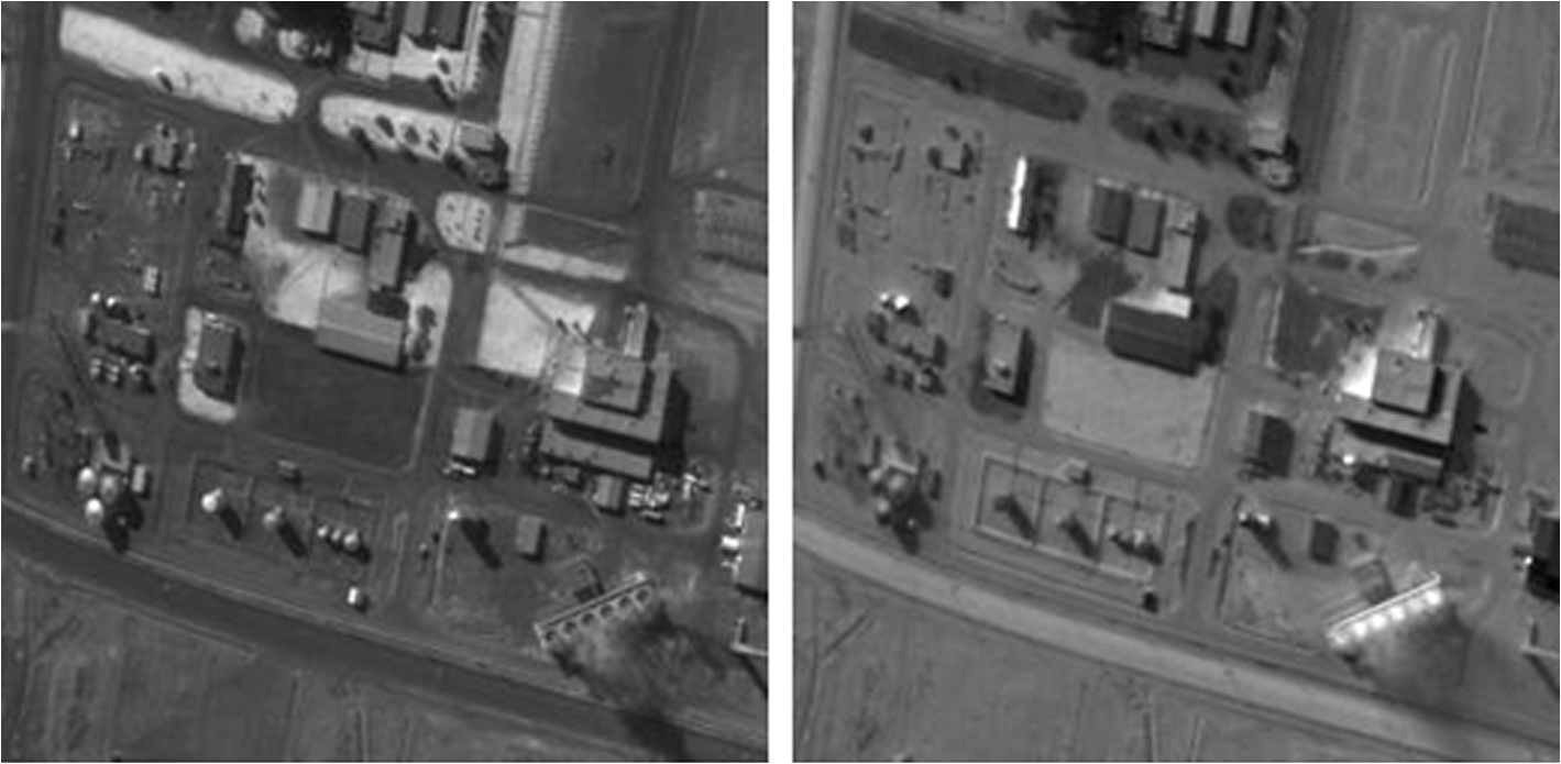
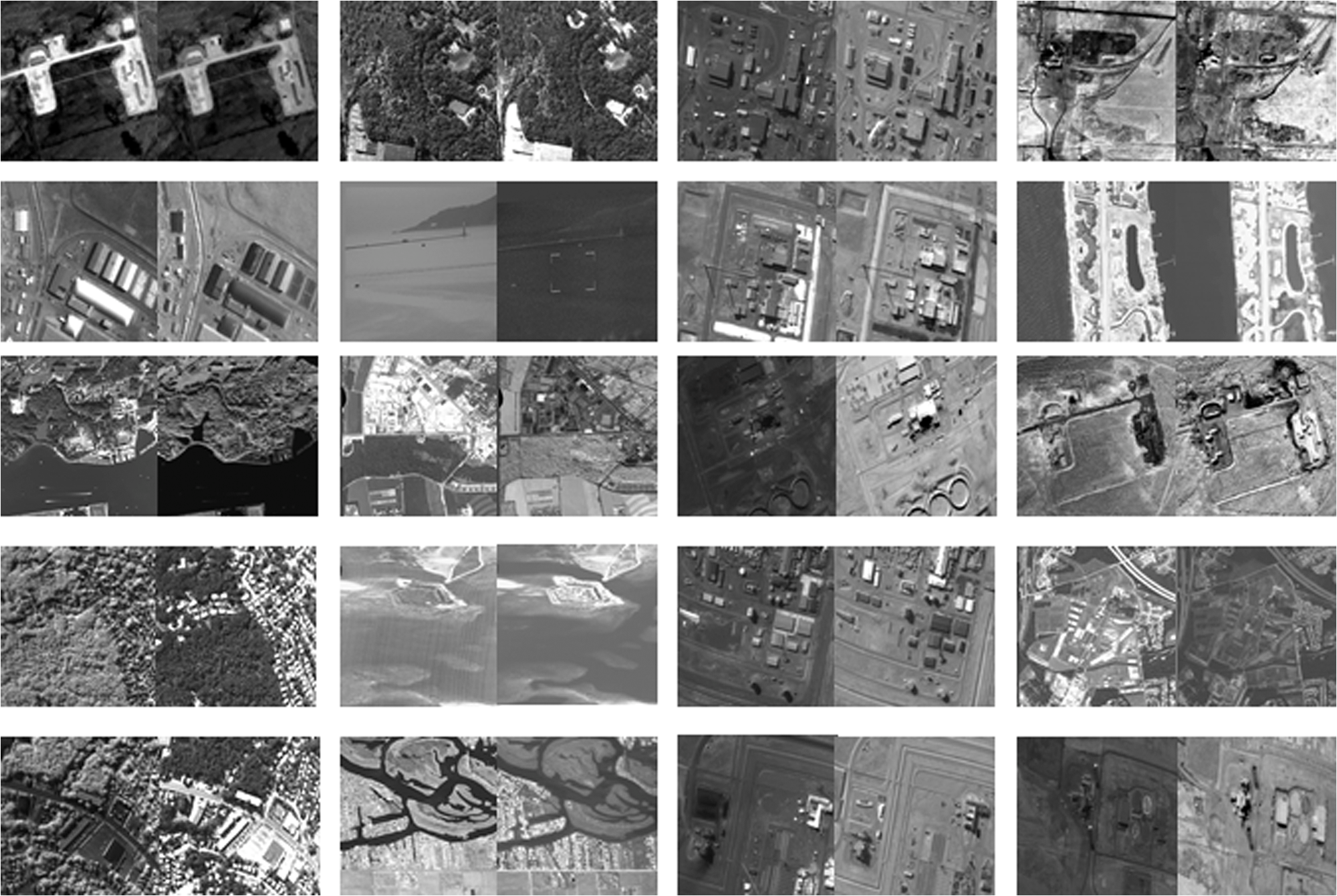
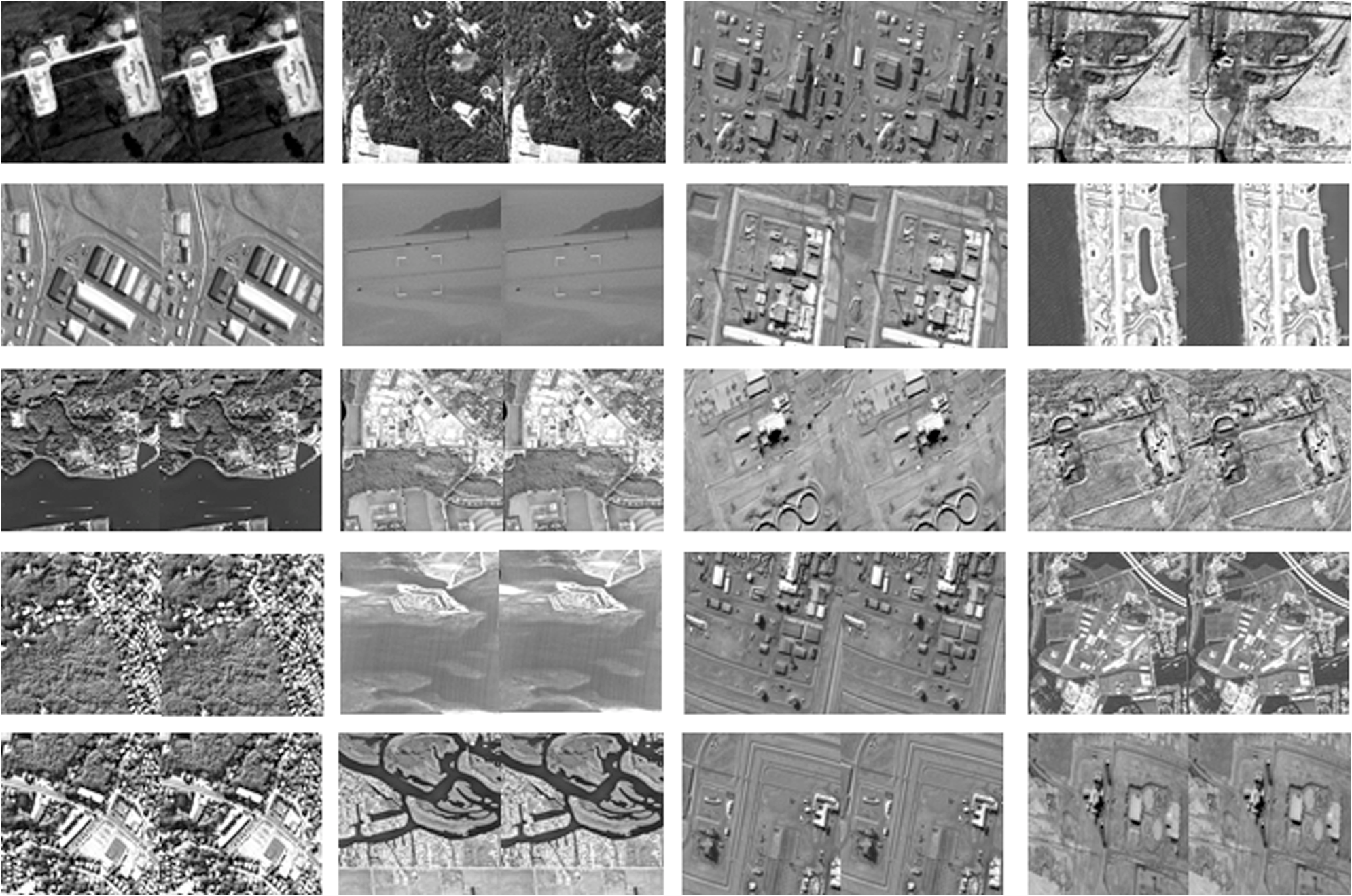
Note: The bold values are the two best results of individual evaluation criteria.

In addition, the complexity of training dictionary in NSCTSR is almost the same as SR, SOMP, and JSR fusion methods, because they all use classical K-SVD dictionary learning method. Although the dictionary of NSCTSR is trained in NSCT domain, the low-pass subband image (coefficients) in NSCT domain is the same size as the source image and the complexity of NSCT decomposition is much smaller than K-SVD algorithm. The dictionary of MODJSR has lower complexity by joint sparse coding and dictionary update stage. The CPU time of the K-SVD and training dictionary in MODJSR and NSCTSR are 108.61, 74.59, and 124.27 s, respectively. However, the dictionary in sparse representation–based fusion method is usually pretrained by using a lot of samples as the number of source images is limited.⁹ Therefore, the complexity of fusion stage in Fig. 5 is more concerned. From the above experiments, it can be seen that the NSCTSR fusion methods with nonoverlapping step exactly decrease the calculation cost of fusion stage.

5.4.

More Results on 20 Pairs of Images

In order to confirm the effectiveness of the proposed method, an experiment on larger image sets is presented. Twenty pairs of multisensor images 001 to 020 from Image Fusion Server are fused by the eight compared methods and NSCTSR, as shown in Fig. 15. Figure 16 illustrates the fused results by NSCTSR, and the step of former image in each set is 1, and the latter one is 8, which is nonoverlapping block approach. We can see that the two kinds of fused results are nearly the same in visual sensation. The objective evaluation of each pairs is calculated, and the average results are shown in Table 5. From Table 5, we observe that the NSCTSR and NSCTSR_S8 method are more effective and superior than other methods. The statistical values demonstrate the superiority of the proposed method.

Fig. 15

Twenty pairs of test images from Image Fusion Server.

Fig. 16

Fused results of the proposed method with one and eight moving steps.

Table 5

Average of the metric over 20 pairs of images.

Methods	$Q_{0}$	$Q_{W}$	$Q_{E}$	$Q_{A B / F}$	$Q_{G}$
DWT	0.6975	0.7384	0.5627	0.5603	0.7535
SWT	0.7462	0.7729	0.6131	0.6002	0.7839
NSCT	0.7632	0.7874	0.6309	0.6284	0.7919
LPSSIM	0.7764	0.7896	0.6249	0.6394	0.7875
SR	0.7665	0.7904	0.6391	0.6390	0.7965
SOMP	0.7587	0.7987	0.6205	0.6452	0.7939
JSR	0.7509	0.7798	0.6204	0.6165	0.7891
MODJSR	0.7790	0.8071	0.6382	0.6473	0.8092
NSCTSR	0.7887	0.8105	0.6414	0.6531	0.8168
NSCTSR_N8	0.7882	0.8101	0.6411	0.6527	0.8139

Note: The bold values are the two best results of individual evaluation criteria.

Table 6 reports the average computation (CPU) time of the above methods. The average CPU time of NSCT and LPSSIM are longer than that of DWT and SWT. The sparse representation–based image fusion methods are much slower than the multiscale transform–based methods because the sliding window scheme with max-overlapping blocks is time-consuming. However, the NSCTSR with nonoverlapping step only takes 15.91 s, without blocking artifacts, which is much faster than other traditional sparse representation–based methods. Although the proposed method takes more time than the muliscale transform-based methods, it gets better results as described above.

Table 6

Average of CPU time of various methods.

Methods	DWT	SWT	NSCT	LPSSIM	SR
CPU time (s)	0.53	0.79	13.79	19.62	85.96
Methods	SOMP	JSR	MODJSR	NSCTSR	NSCTSR_S8
CPU time (s)	73.64	94.15	98.72	87.34	15.91

6. Conclusion

In this paper, we have proposed a fusion method (NSCTSR) based on NSCT and sparse representation. The major contributions of this paper are twofold. First, the salient features of the low-pass subband coefficients in NSCT can be effectively separated through trained dictionary with K-SVD. Meanwhile, the property of multiscale analysis is introduced in sparse representation–based fusion method to improve integrated details. Second, the proposed method with nonoverlapping step can largely decrease the calculation costs than traditional sparse representation methods, without blocking artifacts. The experimental results show that the proposed method has better performance than both multiscale transform–based methods and sparse representation–based methods in the visual effects and quantitative fusion evaluation measures. Furthermore, the NSCTSR is easy to be extended to the existing state-of-the-art NSCT-based image fusion algorithms.

Acknowledgments

The authors would like to thank the anonymous reviewers and editors for their insightful comments and suggestions. This work is supported by the National Nature Science Foundation of China under Grant (61075014,61103062); Aeronautical Science Fund of China(NO.2013ZD53056); The Research Fund for the Doctoral Program of Higher Education(20116102120031); Aerospace Support Fund (2011XW080001C080001); The Doctorate Foundation of Northwestern Polytechnical University (CX201318); NPU Basic Research Foundation (JC201249).

References

1.

G. BhatnagarQ. M. J. WuZ. Liu, “Human visual system inspired multi-modal medical image fusion framework,” Expert Syst. Appl., 40 (5), 1708 –1720 (2013). http://dx.doi.org/10.1016/j.eswa.2012.09.011 ESAPEH 0957-4174 Google Scholar

2.

C. H. Senget al., “Two-stage fuzzy fusion with applications to through-the-wall radar imaging,” IEEE Geosci. Remote Sens., 10 (4), 687 –691 (2013). http://dx.doi.org/10.1109/LGRS.2012.2218570 IGRSD2 0196-2892 Google Scholar

3.

V. S. PetrovicC. S. Xydeas, “Gradient-based multiresolution image fusion,” IEEE Trans. Image Process., 13 (2), 228 –237 (2004). http://dx.doi.org/10.1109/TIP.2004.823821 IIPRE4 1057-7149 Google Scholar

4.

S. C. NercessianK. A. PanettaS. S. Agaian, “Multiscale image fusion using an adaptive similarity-based sensor weighting scheme and human visual system-inspired contrast measure,” J. Electron. Imaging, 21 (2), 021112 (2012). http://dx.doi.org/10.1117/1.JEI.21.2.021112 JEIME5 1017-9909 Google Scholar

5.

Q. GuoS. T. Liu, “Performance analysis of multi-spectral and panchromatic image fusion techniques based on two wavelet discrete approaches,” Optik, 122 (9), 811 –819 (2011). http://dx.doi.org/10.1016/j.ijleo.2010.06.008 OTIKAJ 0030-4026 Google Scholar

6.

S. T. LiJ. T. KwokY. N. Wang, “Discrete wavelet frame transform method to merge Landsat TM and SPOT panchromatic images,” Inf. Fusion, 3 (1), 17 –23 (2002). http://dx.doi.org/10.1016/S1566-2535(01)00037-9 1566-2535 Google Scholar

7.

X. ChangL. C. JiaoJ. H. Jia, “Multisensor image adaptive fusion based on nonsubsampled contourlet,” Chin. J. Comput., 32 (11), 2229 –2237 (2009). Google Scholar

8.

B. YangS. T. Li, “Multifocus image fusion and restoration with sparse representation,” IEEE Trans. Instrum. Meas., 59 (4), 884 –892 (2010). http://dx.doi.org/10.1109/TIM.2009.2026612 IEIMAO 0018-9456 Google Scholar

9.

B. YangS. T. Li, “Pixel-level image fusion with simultaneous orthogonal matching pursuit,” Inf. Fusion, 13 (1), 10 –19 (2012). http://dx.doi.org/10.1016/j.inffus.2010.04.001 1566-2535 Google Scholar

10.

G. YangX. Z. XuH. Man, “Optimum image fusion via sparse representation,” in WOCC 2011-20th Annual Wireless and Optical Communications Conf., (2011). Google Scholar

11.

N. N. YuT. S. QiuF. Bi, “Image features extraction and fusion based on joint sparse representation,” IEEE J. Sel. Topics Signal Process., 5 (5), 1074 –1082 (2011). Google Scholar

12.

Q. H. ZhangY. L. FuH. F. Li, “Dictionary learning method for joint sparse representation-based image fusion,” Opt. Eng., 52 (5), 057006 (2013). http://dx.doi.org/10.1117/1.OE.52.5.057006 OPEGAR 0091-3286 Google Scholar

13.

B. OphirM. LustigM. Elad, “Multi-scale dictionary learning using wavelets,” IEEE J. Sel. Topics Signal Process., 5 (5), 1014 –1024 (2011). Google Scholar

14.

S. T. ShuH. T. YinL. Y. Fang, “Remote sensing image fusion via sparse representations over learned dictionaries,” IEEE Trans. Geosci. Remote Sens., 51 (9), 4779 –4789 (2013). http://dx.doi.org/10.1109/TGRS.2013.2257799 IGRSD2 0196-2892 Google Scholar

15.

M. N. DoM. Vetterli, “The coutourlet transform: an efficient directional multiresolution image representation,” IEEE Trans. Image Process., 14 (12), 2091 –2106 (2005). http://dx.doi.org/10.1109/TIP.2005.859376 IIPRE4 1057-7149 Google Scholar

16.

H. F. LiC. YiZ. F. Li, “Multi-focus fusion based on nonsubsampled contourlet transform and focused regions detection,” Optik, 124 (1), 40 –51 (2013). http://dx.doi.org/10.1016/j.ijleo.2011.11.088 OTIKAJ 0030-4026 Google Scholar

17.

A. L. CunhaJ. ZhouM. N. Do, “The nonsubsampled contourlet transform: theory, design, and applications,” IEEE Trans. Image Process., 15 (10), 3089 –3101 (2006). http://dx.doi.org/10.1109/TIP.2006.877507 IIPRE4 1057-7149 Google Scholar

18.

Q. ZhangB. L. Guo, “Multifocus image fusion using the nonsubsampled contourlet transform,” Signal Process., 89 (7), 1334 –1346 (2009). http://dx.doi.org/10.1016/j.sigpro.2009.01.012 SPRODR 0165-1684 Google Scholar

19.

R. RubinsteinM. ZibulevskyM. Elad, “Double sparsity: learning sparse dictionaries for sparse signal representation,” IEEE Trans. Image Process., 58 (3), 1553 –1564 (2010). http://dx.doi.org/10.1109/TSP.2009.2036477 IIPRE4 1057-7149 Google Scholar

20.

H. T. YinS. T. Li, “Multimodal image fusion with joint sparsity model,” Opt. Eng., 50 (6), 067007 (2011). http://dx.doi.org/10.1117/1.3584840 OPEGAR 0091-3286 Google Scholar

21.

M. AharonM. EladA. Bruckstein, “K-SVD: an algorithm for designing overcomplete dictionaries for sparse representation,” IEEE Trans. Image Process., 54 (11), 4311 –4322 (2006). http://dx.doi.org/10.1109/TSP.2006.881199 IIPRE4 1057-7149 Google Scholar

22.

R. H. LingL. Z. Cheng, “Double sparse image representation via learning dictionaries in wavelet domain,” J. Natl. Univ. Def. Technol., 34 (4), 126 –131 (2012). Google Scholar

23.

Image Fusion Community Website, http://www.Imagefusion.org/ Google Scholar

24.

Z. WangA. C. Bovik, “A universal image quality index,” IEEE Signal Process. Lett., 9 (3), 81 –84 (2002). http://dx.doi.org/10.1109/97.995823 IESPEJ 1070-9908 Google Scholar

25.

G. PiellaH. Heijmans, “A new quality metric for image fusion,” in Proc. of Int. Conf. on Image Processing, 173 –176 (2003). Google Scholar

26.

C. S. XydeasV. Petrovic, “Objective image fusion performance measure,” Electron. Lett., 36 (4), 308 –309 (2000). http://dx.doi.org/10.1049/el:20000267 ELLEAK 0013-5194 Google Scholar

Biography

Jun Wang received her BS degree in telecommunication engineering from North University of China, Taiyuan, China, in 2009 and her MS degrees in circuits and systems from Northwestern Polytechnical University, Xi’an, China, in 2012. She is currently pursuing a PhD degree at the School of Electronics and Information, Northwestern Polytechnical University, Xi’an, China. Her research interests include image processing, sparse representation, and pattern recognition.

Jinye Peng received his MS degree in computer science from Northwestern University, Xi’an, China, in 1996 and his PhD degree from Northwestern Polytechnical University, Xi’an, in 2002. He is with the School of Electronics and Information, Northwestern Polytechnical University, as full-time professor, since 2006. His current research interests include image retrieval, face recognition, and machine learning.

Xiaoyi Feng received her MS degree in computer science from Northwestern University, Xi’an, China, in 1994 and her PhD degree from Northwestern Polytechnical University, Xi’an, in 2001. She is with the School of Electronics and Information, Northwestern Polytechnical University, as full-time professor, since 2009. Her current research interests include image retrieval, face recognition, and computer vision.

Guiqing He received her BS, MS, and PhD degrees in computer science from Northwestern University, Xi’an, China, in 2000, 2005, and 2009, respectively. She is with the School of Electronics and Information, Northwestern Polytechnical University, as associate professor. Her current research interests include data fusion and analyzing and processing of remote sensing image.

Jun Wu received his BS degree in information engineering from Xi’an Jiaotong University in 2001 and his MSc and PhD degrees both in computer science and technology from Tsinghua University in 2004 and in 2008, respectively. He is currently an associate professor in the School of Electronics and Information, Northwestern Polytechnical University. From 2008 to 2010, he was a research staff in the Intelligent Systems Lab Amsterdam of the University of Amsterdam, the Netherlands. During 2003 to 2004, he was a visiting student at Microsoft Research Asia. From August to October in 2005, he was a visiting scholar in the Department of Computer Science, University of Hamburg, Germany. His research interests are in machine learning, multimedia analysis, and multimedia information retrieval.

Kun Yan received his BS and MS degrees in circuits and systems from Northwestern Polytechnical University, Xi’an, China, in 2008 and 2011, respectively. He is with the Institute of Remote Sensing and Data Transmission, China Academy of Space Technology, Xi’an, as an engineer, since 2011. His research interests include processing of remote sensing data, data transmission, and pattern recognition.

CC BY: © The Authors. Published by SPIE under a Creative Commons Attribution 4.0 Unported License. Distribution or reproduction of this work in whole or in part requires full attribution of the original publication, including its DOI.

Citation Download Citation

Jun Wang, Jinye Peng, Xiaoyi Feng, Guiqing He, Jun Wu, and Kun Yan "Image fusion with nonsubsampled contourlet transform and sparse representation," Journal of Electronic Imaging 22(4), 043019 (19 November 2013). https://doi.org/10.1117/1.JEI.22.4.043019

Published: 19 November 2013

Access the abstract

JOURNAL ARTICLE
15 PAGES

DOWNLOAD PAPER SAVE TO MY LIBRARY

GET CITATION

CITATIONS

Cited by 55 scholarly publications.

Explore citations on Lens.org

KEYWORDS

Image fusion

Associative arrays

Stationary wavelet transform

Discrete wavelet transforms

Medical imaging

Chemical species

Visualization

1.

Introduction

2.

Nonsubsampled Contourlet Transform

Fig. 1

Fig. 2

Fig. 3

3.

Sparse Representation in NSCT Domain

3.1.

Sparse Representation for Image Fusion

Eq. (1)

3.2.

Dictionary Learning with K-SVD in NSCT Domain

Eq. (2)

Eq. (3)

Eq. (4)

Eq. (5)

Eq. (6)

Fig. 4

4.

Proposed Image Fusion Scheme

4.1.

Low-Pass Subband Coefficients Fusion

Eq. (7)

Eq. (8)

4.2.

High-Pass Subband Coefficients Fusion

Eq. (9)

Eq. (10)

4.3.

Fusion Scheme

Fig. 5

5.

Experiments

5.1.

Experimental Setup

5.2.

Fusion Results

Fig. 6

Fig. 7

Fig. 8

Table 1

Fig. 9

Fig. 10

Fig. 11

Table 2

5.3.

Discussion on the Sliding Step

Fig. 12

Table 3

Fig. 13

Fig. 14

Table 4

5.4.

More Results on 20 Pairs of Images

Fig. 15

Fig. 16

Table 5

Table 6

6.

Conclusion

Acknowledgments

References

Biography

Show All Keywords

Keywords/Phrases

Search In:

Publication Years