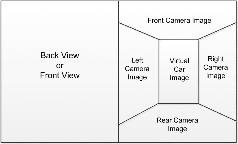
1.1.

State-of-the-Art Technology

Two kinds of parking assistant systems are prevailing in the market. One is parking distance control (PDC), which applies ultrasound transducers, and the other is the video assistant parking system (VAPS), which applies camera sensors.

PDC usually integrates ultrasound transducers into the rear bumpers of automobiles. It measures the distance to the nearest object behind the vehicle and outputs a progressive acoustic warning signal to inform the driver. PDC is able to detect obstacles within 2 m by using ultrasound transducers. However, the exact location, size, and type of obstacles cannot be determined. When the distance between obstacles and the vehicle is below half a meter, the performance of PDC is poor. Although PDC has been well developed by manufacturers in recent years, the main drawback still remains.

A VAPS, which mixes ultrasound transducers with camera sensors, was, therefore, designed and built to overcome the disadvantages of PDC. The system integrates a camera in the rear of the car. When the ultrasound sensor detects an obstacle that is close to the reversing vehicle, the driver can clearly identify what type of obstacle it is. VAPS is limited to visualizing the situation of the rear, and it does not completely solve the occlusion problems that happen at the sides and at the front of the vehicle during parking. Thus, the risk of having parking accidents still exists, even though it is reduced.

A panorama parking system called the around-view monitor and multiview camera system can overcome all the disadvantages of PDC and VAPS; they were first introduced by Nissan together with Xanavi and SONY, and they have been applied in several premium-line vehicle models.

Generally, all panorama parking systems make use of four wide-angle high-resolution cameras. These cameras are installed at the front, the rear, and both sides of a vehicle. Video frames from all these four cameras will be captured and processed. A top-view image will be shown to the driver after processing, allowing the driver to recognize the scenarios of all directions. Because of its high display accuracy that gives in situ views around the car, drivers can park confidently without looking around the car, just looking at the display screen. It not only solves the safety problem, but also makes people drive more easily, even in a complex situation in the parking area or garage. It provides unparalleled advantages compared with PDC and VAPS.

Present performance of panorama parking technologies still has the potential to improve. For instance, the integrity and smoothness of mosaicking images need to be refined by improved algorithms. More importantly, this technology is still very expensive, so it is only employed in original equipment manufacturer (OEM) markets to flagship and high-line vehicle models. It is hard to apply it broadly in normal cars. An after-market solution of this technology with proper price, high performance, and easy installation is necessary for utilization in budget cars, and this is the very purpose of this study.

1.2.

Paper Outline

This paper focuses on the problem of designing an embedded PPAS, which can be applied to most passenger cars with a more accurate and efficient calibration method.

As one subsystem of the advanced driver assistant system for safety, the PPAS should also be designed for easy integration with other subsystems such as the fatigue driving detection system and pedestrian detection system. In this connection, the same system architecture will be employed to facilitate the functional integration.

The PPAS needs to be designed from software to hardware. Fisheye cameras are necessary to cover a proper wide range of views in four directions of the car. Four channels of video will be captured, processed, and stitched to form one smooth top-view image for display on the LCD screen of the automobile. Static or moving objects would be displayed, and the driver will be warned by an audio alert signal if these objects are too close to the car.

From the perspective of algorithm, there are two types of splicing in this paper’s application: the first type is calibrating and optimizing the camera’s parameters, so that the distorted images would be corrected and the prerequisites of routine image splicing methods become available. The second type is to use routine methods to splice the fisheye images corrected by the calibration and optimization methods, and the function of routine splicing methods such as region-based and feature-based methods is to match or splice two pictures’ border. In fact, the routine splicing methods such as region-based and feature-based methods both require that the images have a certain overlapping area and the deformation of the image cannot be too large. Furthermore, they also depend heavily on the position and angle of camera installation. In the case of this paper, all the images captured by fisheye cameras are highly distorted and the position or angle of the cameras would vary greatly when they are installed in different vehicles. So the whole splicing prerequisites in this paper are quite different from the routine splicing methods, such as panorama-photo splicing by iPhone’s function.

In this paper, we mainly focus on the key problem of parameter calibration and optimization because it will decide the efficiency of installing PPAS, which is the key factor to judge the availability of PPAS’s application in 4S shop. Additionally, by the parameter calibration and optimization, the four distorted images would be corrected and have one universal coordinate system, which means that after optimization, the four images could be spliced by coordinates alone.

The paper is, therefore, organized as follows. Section 2 will describe the proposed PPAS. Sections 3 and 4 will describe the general methods of calibration and distortion correction. An improved particle swarm optimization (IPSO) method to optimize calibration will also be described. Section 5 will outline the architecture of the system hardware. Section 6 will describe the implementation results of the system, and finally, Sec. 7 will give the final conclusion of this paper.

3.1.

Projection Transformation

The relationship between the camera coordinate system and world coordinate system can be described by the rotation matrix $R$ and the translation vector $t$. If the homogeneous coordinates of point $P$ in the world coordinate system is ${(X_W,{\mathrm{Y}}_{\mathrm{W}},Z_W,1)}^T$ and the camera coordinate system is ${(x,y,z,1)}^T$, there will be the following relationship:

Considering the relationship of the pixel units and the physical coordinate units, and using a pinhole imaging model and the perspective projection relations, it can be described as follows:

$(x,y,z)$ are the coordinates of point $P$ in the camera coordinate system. $f$ is the distance between the x-y plane and the image plane, which is commonly referred to as the camera focal length; $s$ is the scale factor.

$P$ and its projection coordinates $p(u,v)$ can be expressed as follows:

${\alpha }_x$ and ${\alpha }_y$ are the scale factors and known as the normalized focal length in the $u$-axis and $v$-axis. $M_1\text{'}$ is determined by ${\alpha }_x$,${\alpha }_y$, $u_0$, $v_0$, which is associated with the cameras’ intrinsic parameters.

It is generally assumed that the calibration plane is located on the plane of the world coordinate system. As mentioned in Eq. (1), $R$ is a $3\times 3$ orthogonal matrix and $r$ is the column vector of matrix $R$, and $t$ is the translation vector; therefore, each point on the plane can be described as

The above equation shows the relationship between the point $m={[u,v]}^T$ of the image surface and $M={[X_W,Y_W]}^T$ on the plane.

Then a single mapping matrix $H$ (Ref. 10) is established between the pixel point and the point on a plane template, as follows:

3.2.

Solution for Intrinsic and Extrinsic Parameters

The constraint equation for intrinsic parameters is from Eq. (5). It is shown as follows:

Because $R$ is the orthogonal matrix, two basic constraints of the intrinsic parameters can be deduced as

In order to get a linear solution for camera intrinsic parameters, we assume

$B$ is a symmetric matrix and can be defined as vector $b$,

So $h_i^{T}B{h}_j=v_{ij}^{T}b$ is obtained; then revise the constraint equations into two vector equations as follows:

If there are $n$ template plane images as parameters, use Eq. (10) to obtain the solutions. If $n\ge 3$, the eigenvector corresponding to a minimum eigenvalue of V is the solution of this equation. ¹¹ Once vector b is obtained, the intrinsic parameter matrix $M_1^{-1}$ can be obtained by the Cholesky decomposition.

Then the inverse matrix is the camera’s intrinsic parameters matrix $M_1^{-1}$, which can deduce the solution of intrinsic parameters as follows:

The extrinsic parameters of each image that correspond to the plane template can be calculated by the following equations:

3.3.

Optimization of the Linear Calibration Results

Due to the structure and installation error of the lens, there would be some distortion in the image. In order to improve the accuracy of the calibration, considering the radial and tangential distortion of the lens, an equation was applied as follows:^12,13

Considering both the extrinsic and intrinsic parameters as unknown parameters and calculating them, a nonlinear equation can be obtained. Suppose there are $n$ images that correspond to the template plane and $m$ calibration points in the template plane, a cost function can be described as follows:

$m(A,k_1,k_2,p_1,p_2,R_i,t_i,M_j)$ is a pixel coordinate obtained by known parameters, $A$ is the matrix of intrinsic parameters, and $k_1,k_2,p_1,p_2$ are distortion parameters. The optimal solution of this problem is to minimize the cost function.

The Levenberg-Marquadt algorithm is applied to solve the nonlinear least-squares problem. The initial estimated values are the results of the above linear solution.^14,15

4.1.

Particle Swarm Optimization Algorithm

PSO was proposed by Kennedy and Eberhart;¹⁶ it is a stochastic optimization method based on swarm intelligence theory. It has been successfully applied in continuous optimization problems such as neural network training, voltage stability control, and the optimization of cutting parameters.

The main idea is to simulate the intelligent behavior of an individual particle in a swarm, just like an individual bird searching for food in a group or population. By group cooperation, the swarm can get maximum global optimization results.^17,18 In this paper the PSO method is applied to get the maximum optimized intrinsic or extrinsic global parameters of the fisheye camera so as to make the mosaicking function available by efficient calibration when installing PPAS in 4S shops.

The particle is the basic unit of the algorithm, and in the optimization problem, it is a candidate solution of the D-dimensional space. Assume the solution vector is D-dimensional and the total number of particles is $n$. When the algorithm iterates $t$ times, the $i$’th particle can be expressed as

Individual extreme $p_i=[p_{i1},p_{i2},\dots ,p_{\mathrm{id}}]$ is the most optimal solution vector of a single particle from the initial search to the current iteration.

Neighborhood extreme $l_i=[l_{i1},l_{i2},\dots ,l_{\mathrm{id}}]$ is the most optimal solution vector of a particle’s corresponding neighborhood population from the initial search to the current iteration.

Particle velocity $v_i(t)=[v_{i1}(t),v_{i2}(t),\dots ,v_{\mathrm{id}}(t)]$ represents a particle’s changes in the location within the unit iteration number, that is, it is a particle’s displacement of the solution variable in D-dimensional space, where $v_{ik}(t)$ represents the velocity of the $i$’th particle in the $k$-dimensional solution space.

The inertia weight $w$ is used to control how much the speed of the previous iteration affects the current iterative speed. Generally, inertia weight is $w\in [0,1]$. Shi and Eberhart found that a larger inertia weight is conducive to a global search in particle population, while a smaller inertia weight is inclined to a local search.¹⁹ In the actual solving process of the optimization problem, the inertia weight is decreasing linearly with the iteration number $w(t)=a\times w(t-1)$. Therefore, in the initial search stage of this case, the search of the whole solution space can be carried out with high probability and can converge quickly to the optimal solution in a local area, where the local fine-tuning for particle population can be finished with the decrease of the inertia weight.

PSO first initializes a random particle population (random solution) and then searches the optimal solution by iteration. The particle updates its location and velocity through individual extremes and neighborhood extremes on every iteration.

The location of each particle changes according to the following equations:^20,21

4.2.

Improved Particle Swarm Optimization Algorithm

The ordinary PSO algorithm is only an evolutionary mechanism, whose emphasis is more on groups to optimize or develop individuals. The traditional PSO methods have the advantage due to their good global convergence speed with a better solution; however, their disadvantage is that they easily fall into local optimum.

For the improvement of ordinary PSO, using PSO at the basis of a two-step method is applied by many people. First, the PSO method is used to do a global search, and then a second algorithm is applied which is good at processing locally. The solution obtained by PSO is regarded as the initial solution for further optimization. The problem is that after the global convergence, the solution is difficult to jump out of the region convergence. In conclusion, the conventional two-step method is better than routine PSO, but it still cannot improve the performance of PSO, essentially because it has been assumed that the PSO convergence region belongs to the optimal region. For example, there are three zones ($A$, $B$, and $C$) in the solution set—$A_{\text{best}}$, $B_{\text{best}}$, and $C_{\text{best}}$ belong to $A$, $B$, and $C$, respectively. $C_{\text{best}}$ is better than $B_{\text{best}}$, and $B_{\text{best}}$ is better than $A_{\text{best}}$; if the PSO method could only find $B_1$, the second algorithm would definitely find ${\mathrm{B}}_{\text{best}}$, yet it has not jumped out of $B$ to find the best solution in the optimal $C$ zone. By this way, all particles only rely on the good information, which means the particle moves to the best position in the local or global area. That would be premature aggregation and lost diversity and it would not be the best optimization.

Apart from this, the real working situation required the applied method to meet the following conditions:

The method relying on multiple images or the edge-based method can hardly be applied in this situation. Therefore, to find a way to calibrate or optimize all the parameters with only one reference image and not be influenced by the working environment is important, because it will make calibration and optimization available in all kinds of work fields in the 4S shops.

An IPSO algorithm is, therefore, proposed to optimize the parameters, considering the above conditions.

The proposed IPSO method is able to break the convergence space for it has two mechanisms: toward the best and away from the worst. Both mechanisms are toward the right direction. The convergence rate of the algorithm maintains the same high efficiency, although it is not allowed to converge toward a single direction in which it will be trapped in the local solution, so as to find the global optimum.

When using a method relying on multiple images and edge-based method, the edges have to be determined manually if the edge cannot be detected. The IPSO allows a certain range of dynamic change for the parameters; it can exploit only one reference image to complete all the calibration or optimization without extra manual operation. That makes IPSO suitable in practical application in the workshop with light-changing conditions with a minimum of reference images.

If good and bad information are both taken into account in the algorithm to add a method of changing in velocity, the case will change when introducing the following equation:

Population density is introduced; if the density is low, it means the direction of evolution is good, so Eq. (18) is applied. If the density is high, it means the direction of the evolution is approaching the bad side, so Eq. (20) is applied. Diversity($P$) is the measure of the density; the greater the density is, the lower the value of diversity($P$) is. Its equation is as follows:²³

$|L|$ is the size of the search space, $S\in R^N$, $N$ is the number of dimensions, $S_{ij}$ is the value of the $i$’th particle in the n$j$’th dimension, and ${\overline{S}}_j$ is the average value of a particle in the $j$’th dimension.

In the PSO algorithm, the velocity $v$ is used to promote the evolution of the particle population; however, this mechanism only works on specific particles, and when the particles tend to gather, the population can easily lose its vitality.

Increasing the uncertainty of the particle motion means the particle has a random nature. This can make the whole population maintain vitality. A variation will be introduced to the PSO, and Eq. (19) will be changed as follows:

The IPSO method has two phases: first, the particle is attracted by the best position, and second, it will be pushed away from the worst position. This mechanism means the particle moves to the good position or a “not bad” position. For the change of the particle reference, the swarm or group can leave the local optimum with the maximum probability. In IPSO, the mutation factor is introduced to enhance the vitality of the group.

From the process described above, it can be seen that the IPSO finds the optimized solution by iteration. This character makes it available to apply only one reference image to finish the whole optimization process without being influenced by the environment. That is the reason IPSO is proposed. The effect of the IPSO algorithm with the mutation operator is better than the traditional PSO algorithm, but the result is still not satisfactory, it still leaves room for improvement.

After parameter calibration and optimization, the four distorted images would be corrected and have one universal coordinate system. Therefore, the four images applied in this application could be spliced by coordinates alone. Because the scene in this paper is also comparatively small and easy to mosaic by coordinates, some more complex region-based and feature-based splicing methods are not further compared after the process of calibration and optimization.

6.1.

Result of Fisheye Camera Calibration

In the fisheye calibration step, Zhang’s two-step method and polynomial coordinate transformation method are applied. The calibration needs at least three images with different shooting angles. In this study, nine chessboard-like images with $8\times 8$ grids shooting from different directions are used for the calibration. Forty-nine corners need to be detected. An improved chess corner detection function is applied for the detection; it can get a better result when the fisheye distortion is bigger or the quality of the image is not good. Figure 6 shows the chess corners detected by this improved function.

Fig. 6

The corners detected by the program.

Use the image with the detected chess corners to calibrate the fisheye camera. In order to increase the accuracy of the result, a recalibration step based on former calibration is necessary.

To test the accuracy, an inverse projection of the grid corner procedure is applied, as shown in Fig. 7, where the $\text{character}+\text{represents}$ the detected corners and the circle character indicates the corner location by inverse projection. The figure shows that the calibrated locations of the corners are fit for the original locations.

Fig. 7

Image points and reprojected grid points.

The errors for the inverse projection of different images are shown in Fig. 8. The average range of errors in the distortion correction is generally within one pixel, thereby meeting the basic functional needs of the system.

Fig. 8

The error map of inverse projection.

Figure 9 is the result of the correction of the fisheye camera distortion after basic calibration.

Fig. 9

The result of correction of the fisheye camera distortion after basic calibration.

6.2.

Result of Image Mosaicking

In this study, image mosaicking can be considered the problem of parameter optimization. When the parameter calibration of the four cameras around the vehicle is finished and the errors are minimized in global, the four images are blended.

Besides errors of intrinsic parameters due to manufacturing tolerance, the installation technique of different workers also contributes deviations to the intrinsic parameters. Therefore, the parameter calibration according to the standard reference parameters is necessary in IPSO optimization. It would increase the installation and calibration efficiency in the production line, meanwhile maintaining the same high accuracy.

Four templates are used in the experiments to analyze and compare the results of three algorithms—traditional PSO, IPSO, and PSO—with a mutation operator.

In this study, the angle of the fisheye camera lens is $>165\mathrm{deg}$. According to the result of experiments, the standard reference intrinsic parameters in this paper are regulated as

The four fisheye cameras have two sets of extrinsic parameters for their locations. One set corresponds to the front and the rear cameras, and the other set corresponds to the cameras on both sides of the vehicle.

The front/back cameras’ extrinsic parameters are set as

With these reference parameters, the PPAS will be calibrated with a black and white chessboard-like map as a reference to get preferable optimized parameters.

Three workers were arranged to calibrate the side and the front/back cameras, and got a serial of experiment data to be evaluated. As Eq. (15) described, the optimization problem can be considered to minimize the difference of the rebuilt image and the original one, so the evaluation criteria can be defined as follows.

Using Eq. (15) to calculate the ratio of the minh and the total pixel of the template, if the ratio is $<6\%$, it is defined as success. Calculate the ratio of the success number and the total calibration number. It is defined as the success rate.

The success rate of these three methods is compared in Table 1. Eight pictures were taken for the experiments and each picture was performed for 10 tests for the experiments, and the number 1,2,3,4,5,6 is the number of six selected experimental pictures. From the table, it can be seen that the success rate of the IPSO with a mutation operator is better than the other two methods and that it meets the demands of the PPAS system.

Table 1

Comparison of three methods’ success rate.

Besides the price factor, the convenience of the installation is another key problem for PPAS utilization in the mass market. The most time-consuming step in installation is camera calibration because it has to take into account all the errors accumulated in every manufacture and installation step to ensure the accuracy of mosaicking.

Table 2 shows the average calibration time of IPSO. The tests are based on three sets of experiments upon three different cars of the same type. From the table it can be seen that the average calibration time of each camera is $<3\min$. Compared with manual calibration, the efficiency was increased more than twice.

Table 2

The average calibration time of IPSO.

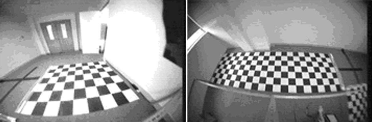
Table 3 shows one set of optimized parameters of the front and the side fisheye cameras by the IPSO method; it is the result of one specific brand of car made by Dongfeng Nissan. Two original images captured by the fisheye cameras in the experiment are shown in Fig. 10.

Table 3

Parameters optimized by IPSO.

Fig. 10

The original images.

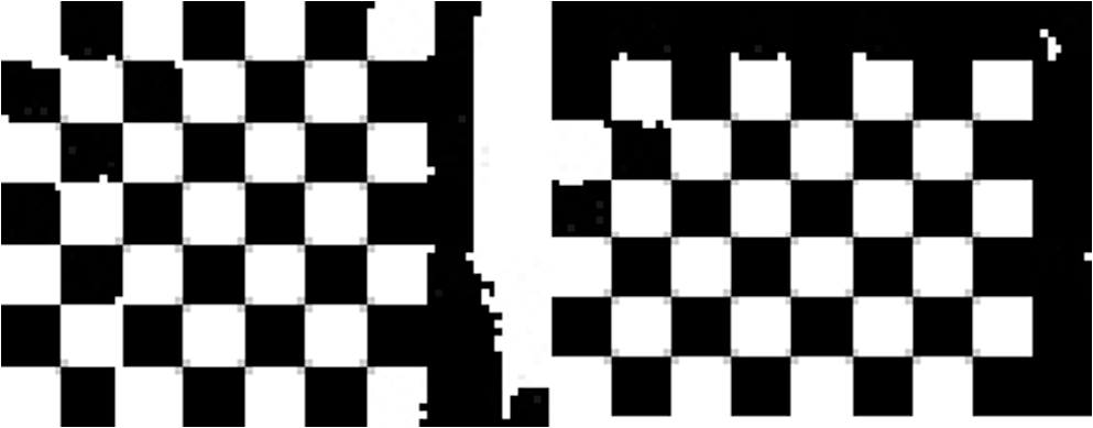
The images with initial external parameters set by PSO are shown in Fig. 11.

Fig. 11

Top-view image with initial external parameter.

The image optimized by IPSO is shown in Fig. 12, and it is the image of the local optimal solution. Figure 13 is the maximum top view using the optimized extrinsic parameters.

Fig. 12

Local optimal solution obtained by improved particle swarm optimization.

Fig. 13

The maximum top view using the optimized extrinsic parameters.

After the calibration of the cameras, a more initial way to judge the effect of the calibration is to restore the images captured by the fisheye camera into a 2-D top-view image. The mosaicking effect can be judged by evaluation criteria mentioned above; if ratio $L$ is $<6\%$, the result is preferred.

The ultimate top mosaicking view is shown in Fig. 14. The ratio $L$ of the image in Fig. 17 is $<6\%$, and from the figure, it can be seen that the four restored images are well spliced. The deviation of $+$ at the joints of the two neighbor images are very small. It is available enough for PPAS.

Fig. 14

Top view after mosaicking.

6.3.

Real Car Test

The PPAS has been installed and tested in several types of cars to test its performance.

Figure 15 shows the performance of the first version of the PPAS prototype installed in a Nissan NV200. It was tested on the basketball ground outside the workshop to see the continuity of the curve after image mosaicking. The figure shows that the curve can almost be connected seamlessly. The test video is Video 1.

Fig. 15

Top-view image from the first version of PPAS prototype (Video 1, MPEG, 11.3 MB) [URL: http://dx.doi.org/10.1117/1.JEI.22.4.041123.1.].

Figure 16 shows the performance of the final version of the PPAS. The system algorithm was upgraded in a seamless connection by applying the weighted smoothing method;²⁴ therefore the four images blocks mosaicked by coordinates were further made seamless in borders.

Fig. 16

Top-view image after mosaicking in final version of PPAS.

Figure 17 shows the mosaicking effect comparison of different brands of car. Figure 17(a) is the effect of Infiniti’s around-view system, Fig. 17(b) is the mosaicking effect of the Honda multiview system, Fig. 17(c) is the effect of BMW 5 serial’s parking assistant system, and Fig. 17(d) is the mosaicking effect of the proposed PPAS in this paper.

Fig. 17

Top-view effect of different types of car.

The PPAS was also installed in other types of automobile and can be widely used in the after-auto market for family cars. The wide application of a similar system would greatly improve parking safety, especially for children, which is the purpose of this study.