Book Review: Compressive sensing for through-the-wall radar imaging

Moeness G. Amin; Fauzia Ahmad

doi:10.1117/1.JEI.22.3.030901

1 July 2013 Compressive sensing for through-the-wall radar imaging

Moeness G. Amin, Fauzia Ahmad

Author Affiliations +

Journal of Electronic Imaging, Vol. 22, Issue 3, 030901 (July 2013). https://doi.org/10.1117/1.JEI.22.3.030901

Abstract

Through-the-wall radar imaging (TWRI) is emerging as a viable technology for providing high-quality imagery of enclosed structures. TWRI makes use of electromagnetic waves to penetrate through building wall materials. Due to the “see” through ability, TWRI has attracted much attention in the last decade and has found a variety of important civilian and military applications. Signal processing algorithms have been devised to allow proper imaging and image recovery in the presence of high clutter, which is caused by front walls and multipath due to reflections from internal walls. Recently, research efforts have shifted toward effective and reliable imaging under constraints on aperture size, frequency, and acquisition time. In this respect, scene reconstructions are being pursued with reduced data volume and within the emerging compressive sensing (CS) framework. We present a review of the CS-based scene reconstruction techniques that address the unique challenges associated with fast and efficient imaging in urban operations. Specifically, we focus on ground-based imaging systems for indoor targets. We discuss CS-based wall mitigation, multipath exploitation, and change detection for imaging of stationary and moving targets inside enclosed structures.

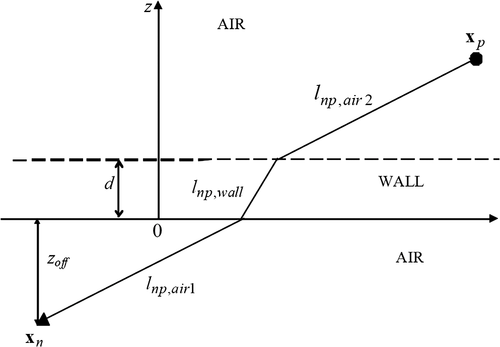
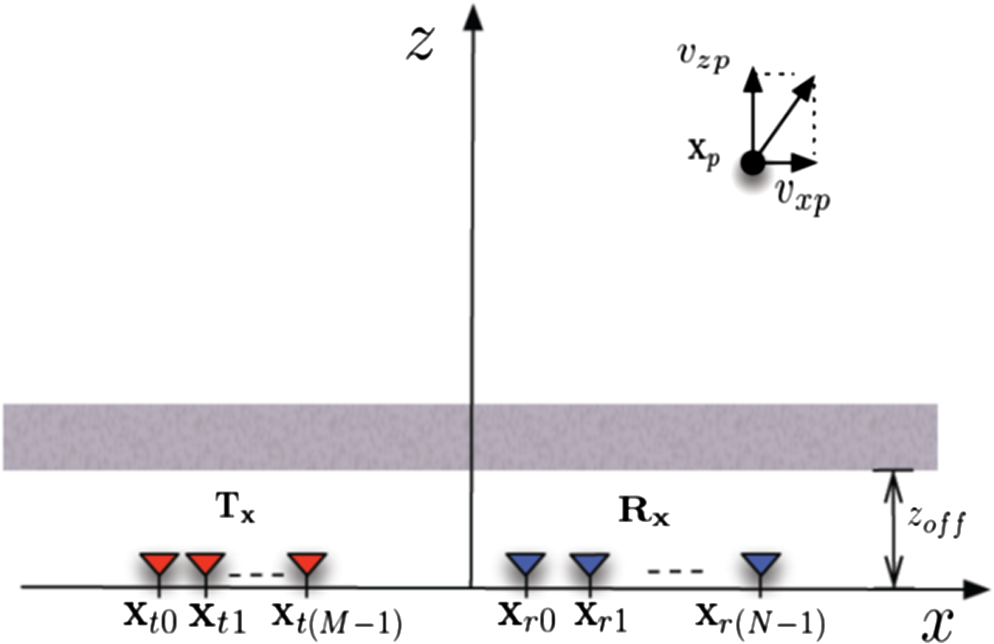
1. Introduction

Through-the-wall radar imaging (TWRI) is an emerging technology that addresses the desire to see inside buildings using electromagnetic (EM) waves for various purposes, including determining the building layout, discerning the building intent and nature of activities, locating and tracking the occupants, and even identifying and classifying inanimate objects of interest within the building. TWRI is highly desirable for law enforcement, fire and rescue, and emergency relief, and military operations.¹^–⁶

Applications primarily driving TWRI development can be divided based on whether information on motions within a structure or on imaging the structure and its stationary contents is sought out. The need to detect motion is highly desirable to discern about the building intent and in many fire and hostage situations. Discrimination of movements from background clutter can be achieved through change detection (CD) or exploitation of Doppler.⁷^–²⁴ One-dimensional (1-D) motion detection and localization systems employ a single transmitter and receiver and can only provide range-to-motion, whereas two- and three-dimensional (2-D and 3-D) multi-antenna systems can provide more accurate localization of moving targets. The 3-D systems have higher processing requirements compared with 2-D systems. However, the third dimension provides height information, which permits distinguishing people from animals, such as household pets. This is important since radar cross-section alone for behind-the-wall targets can be unreliable.

Imaging of structural features and stationary targets inside buildings requires at least 2-D and preferably 3-D systems.²⁵^–⁴³ Because of the lack of any type of motion, these systems cannot rely on Doppler processing or CD for target detection and separation. Synthetic aperture radar (SAR) based approaches have been the most commonly used algorithms for this purpose. Most of the conventional SAR techniques usually neglect propagation distortions such as those encountered by signals passing through walls.⁴⁴ Distortions degrade the performance and can lead to ambiguities in target and wall localizations. Free-space assumptions no longer apply after the EM waves propagate through the first wall. Without factoring in propagation effects, such as attenuation, reflection, refraction, diffraction, and dispersion, imaging of contents within buildings will be severely distorted. As such, image formation methods, array processing techniques, target detection, and image sharpening paradigms must work in concert and be reexamined in view of the nature and specificities of the underlying sensing problem.

In addition to exterior walls, the presence of multipath and clutter can significantly contaminate the radar data leading to reduced system capabilities for imaging of building interiors and localization and tracking of targets behind walls. The multiple reflections within the wall result in wall residuals along the range dimension. These wall reverberations can be stronger than target reflections, leading to its masking and undetectability, especially for weak targets close to the wall.⁴⁵ Multipath stemming from multiple reflections of EM waves off the targets in conjunction with the walls may result in the power being focused at pixels different than those corresponding to the target. This gives rise to ghosts, which can be confused with the real targets inside buildings.⁴⁶^–⁴⁹ Further, uncompensated refraction through walls can lead to localization or focusing errors, causing offsets and blurring of imaged targets.²⁶^,³⁹ SAR techniques and tomographic algorithms, specifically tailored for TWRI, are capable of making some of the adjustments for wave propagation through solid materials.²⁶^–³⁰^,³⁶^–⁴¹^,⁵⁰^–⁵⁷ While such approaches are well suited for shadowing, attenuation, and refraction effects, they do not account for multipath as well as strong reflections from the front wall.

The problems caused by the front wall reflections can be successfully tackled through wall clutter mitigation techniques. Several approaches have been devised, which can be categorized into those based on estimating the wall parameters and others incorporating either wall backscattering strength or invariance with antenna location.³⁹^,⁴⁵^,⁵⁸^–⁶¹ In Refs. 39 and 58, a method to extract the dielectric constant and thickness of the nonfrequency dependent wall from the time-domain scattered field was presented. The time-domain response of the wall was then analytically modeled and removed from the data. In Ref. 45, a spatial filtering method was applied to remove the DC component corresponding with the constant-type radar return, typically associated with the front wall. The third method, presented in Refs. 59–61, was based not only on the wall scattering invariance along the array but also on the fact that wall reflections are relatively stronger than target reflections. As a result, the wall subspace is usually captured in the most dominant singular values when applying singular value decomposition (SVD) to the measured data matrix. The wall contribution can then be removed by orthogonal subspace projection.

Several methods have also been devised for dealing with multipath ghosts in order to provide proper representation of the ground truth. Earlier work attempted to mitigate the adverse effects stemming from multipath propagation.²⁷ Subsequently, research has been conducted to utilize the additional information carried by the multipath returns. The work in Ref. 49 considered multipath exploitation in TWRI, assuming prior knowledge of the building layout. A scheme taking advantage of the additional energy residing in the target ghosts was devised. An image was first formed, the ghost locations for each target were calculated, and then the ghosts were mapped back onto the corresponding target. In this way, the image became ghost-free with increased signal-to-clutter ratio (SCR).

More recently, the focus of the TWRI research has shifted toward addressing constraints on cost and acquisition time in order to achieve the ultimate objective of providing reliable situational awareness through high-resolution imaging in a fast and efficient manner. This goal is primarily challenged due to use of wideband signals and large array apertures. Most radar imaging systems acquire samples in frequency (or time) and space and then apply compression to reduce the amount of stored information. This approach has three inherent inefficiencies. First, as the demands for high resolution and more accurate information increase, so does the number of data samples to be recorded, stored, and subsequently processed. Second, there are significant data redundancies not exploited by the traditional sampling process. Third, it is wasteful to acquire and process data samples that will be discarded later. Further, producing an image of the indoor scene using few observations can be logistically important, as some of the measurements in space and frequency or time can be difficult, unavailable, or impossible to attain.

Toward the objective of providing timely actionable intelligence in urban environments, the emerging compressive sensing (CS) techniques have been shown to yield reduced cost and efficient sensing operations that allow super-resolution imaging of sparse behind-the-wall scenes.¹⁰^,⁶²^–⁷⁶ Compressive sensing is an effective technique for scene reconstruction from a relatively small number of data samples without compromising the imaging quality.⁷⁷^–⁸⁹ In general, the minimum number of data samples or sampling rate that is required for scene image formation is governed by the Nyquist theorem. However, when the scene is sparse, CS provides very efficient sampling, thereby significantly decreasing the required volume of data collected.

In this paper, we focus on CS for TWRI and present a review of $l_{1}$ norm reconstruction techniques that address the unique challenges associated with fast and efficient imaging in urban operations. Sections 2 3 4–5 deal with imaging of stationary scenes, whereas moving target localization is discussed in Sec. 6 and 7. More specifically, Sec. 2 deals with CS based strategies for stepped-frequency based radar imaging of sparse stationary scenes with reduced data volume in spatial and frequency domains. Prior and complete removal of clutter is assumed, which renders the scene sparse. Section 3 presents CS solutions in the presence of front wall clutter. Wall mitigation in conjunction with application of CS is presented for the case when the same reduced frequency set is used from all of the employed antennas. Section 4 considers imaging of the building interior structures using a CS-based approach, which exploits prior information of building construction practices to form an appropriate sparse representation of the building interior layout. Section 5 presents CS based multipath exploitation technique to achieve good image reconstruction in rich multipath indoor environments from few spatial and frequency measurements. Section 6 deals with joint localization of stationary and moving targets using CS based approaches, provided that the indoor scene is sparse in both stationary and moving targets. Section 7 discusses a sparsity-based CD approach to moving target indication for TWRI applications, and deals with cases when the heavy clutter caused by strong reflections from exterior and interior walls reduces the sparsity of the scene. Concluding remarks are provided in Sec. 8. It is noted that for the sake of not overcomplicating the notation, some symbols are used to indicate different variables over different sections of the paper. However, for those cases, these variables are redefined to reflect the change.

The progress reported in this paper is substantial and noteworthy. However, many challenging scenarios and situations remain unresolved using the current techniques and, as such, further research and development are required. However, with the advent of technology that brings about better hardware and improved system architectures, opportunities for handling more complex building scenarios will definitely increase.

2. CS Strategies in Frequency and Spatial Domains for TWRI

In this section, we apply CS to through-the-wall imaging of stationary scenes, assuming prior and complete removal of the front wall clutter.⁶²^,⁶³ For example, if the reference scene is known, then background subtraction can be performed for removal of wall clutter, thereby improving the sparsity of the behind-the-wall stationary scene. We assume stepped-frequency-based SAR operation. We first present the through-the-wall signal model, followed by a description of the sparsity-based scene reconstruction, highlighting the key equations. It is noted that the problem formulation can be modified in a straightforward manner for pulsed operation and multistatic systems.

2.1.

Through-the-Wall Signal Model

Consider a homogeneous wall of thickness $d$ and dielectric constant $ε$ located along the $x$ -axis, and the region to be imaged located beyond the wall along the positive $z$ -axis. Assume that an $N$ -element line array of transceivers is located parallel to the wall at a standoff distance $z_{off}$ , as shown in Fig. 1. Let the $n$ ’th transceiver, located at $x_{n} = (x_{n}, - z_{off})$ , illuminate the scene with a stepped-frequency signal of $M$ frequencies, which are equispaced over the desired bandwidth $ω_{M - 1} - ω_{0}$ ,

Eq. (1)

ω_{m} = ω_{0} + m Δ ω, m = 0, 1, \dots, M - 1,

where

ω_{0}

is the lowest frequency in the desired frequency band and

Δ ω

is the frequency step size. The reflections from any targets in the scene are measured only at the same transceiver location. Assuming the scene contains

P

point targets and the wall return has been completely removed, the output of the

n

’th transceiver corresponding to the

m

’th frequency is given by

Eq. (2)

y (m, n) = \sum_{p = 0}^{P - 1} σ_{p} \exp (- j ω_{m} τ_{p, n}),

where

σ_{p}

is the complex reflectivity of the

p

’th target, and

τ_{p, n}

is the two-way traveling time between the

n

’th antenna and the target. It is noted that the complex amplitude due to free-space path loss, wall reflection/transmission coefficients and wall losses, is assumed to be absorbed into the target reflectivity. The propagation delay

τ_{p, n}

is given by²⁷^–²⁸^,⁴⁰

Eq. (3)

τ_{p, n} = \frac{2 l_{n p, air, 1}}{c} + \frac{2 l_{n p, wall}}{υ} + \frac{2 l_{n p, air, 2}}{c},

where

c

is the speed of light in free-space,

υ = c / \sqrt{ε}

is the speed through the wall, and the variables

l_{n p, air, 1}

,

l_{n p, wall}

, and

l_{n p, air, 2}

represent the traveling distances of the signal before, through, and beyond the wall, respectively, from the

n

’th transceiver to the

p

’th target.

Fig. 1

Geometry on transmit of the equivalent two-dimensional (2-D) problem.

An equivalent matrix-vector representation of the received signals in Eq. (2) can be obtained as follows. Assume that the region of interest is divided into a finite number of pixels $N_{x} \times N_{z}$ in cross-range and downrange, and the point targets occupy no more than $P (≪ N_{x} \times N_{z})$ pixels. Let $r (k, l)$ , $k = 0, 1, \dots, N_{x} - 1$ , $l = 0, 1, \dots, N_{z} - 1$ , be a weighted indicator function, which takes the value $σ_{p}$ if the $p$ ’th point target exists at the $(k, l)$ ’th pixel; otherwise, it is zero. With the values $r (k, l)$ lexicographically ordered into a column vector $r$ of length $N_{x} N_{z}$ , the received signal corresponding to the $n$ ’th antenna can be expressed in matrix-vector form as

Eq. (4)

y_{n} = Ψ_{n} r,

where

Ψ_{n}

is a matrix of dimensions

M \times N_{x} N_{z}

, and its

m

’th row is given by

Eq. (5)

{[Ψ_{n}]}_{m} = [\begin{matrix} e^{- j ω_{m} τ_{00, n}} & \dots & e^{- j ω_{m} τ_{(N_{x} N_{z} - 1), n}} \end{matrix}] .

Considering the measurement vector corresponding to all

N

antennas, defined as

Eq. (6)

y = {[y_{0}^{T} y_{1}^{T} \dots y_{N - 1}^{T}]}^{T},

the relationship between

y

and

r

is given by

Eq. (7)

y = Ψ r,

where

Eq. (8)

Ψ = {[Ψ_{0}^{T} Ψ_{1}^{T} \dots Ψ_{N - 1}^{T}]}^{T} .

The matrix

Ψ

is a linear mapping between the full data

y

and the sparse vector

r

.

2.2.

Sparsity-Based Data Acquisition and Scene Reconstruction

The expression in Eq. (7) involves the full set of measurements made at the $N$ array locations using the $M$ frequencies. For a sparse scene, it is possible to recover $r$ from a reduced set of measurements. Consider $\overset{̆}{y}$ , which is a vector of length $Q_{1} Q_{2} (≪ M N)$ consisting of elements chosen from $y$ as follows:

Eq. (9)

\overset{̆}{y} = Φ y = Φ Ψ r,

where

Φ

is a

Q_{1} Q_{2} \times M N

matrix of the form,

Eq. (10)

Φ = kron (ϑ, I_{Q_{1}}) \cdot diag {φ^{(0)}, φ^{(1)}, \dots, φ^{(N - 1)}} .

In Eq. (10), kron denotes the Kronecker product,

I_{Q_{1}}

is a

Q_{1} \times Q_{2}

identity matrix,

ϑ

is a

Q_{2} \times N

measurement matrix constructed by randomly selecting

Q_{2}

rows of an

N \times N

identity matrix, and

φ^{(n)}

,

n = 0, 1, \dots, N - 1

, is a

Q_{1} \times M

measurement matrix constructed by randomly selecting

Q_{1}

rows of an

M \times M

identity matrix. We note that

ϑ

determines the reduced antenna locations, whereas

φ^{(n)}

determines the reduced set of frequencies corresponding to the

n

’th antenna location. The number of measurements

Q_{1} Q_{2}

required to achieve successful CS reconstruction highly depends on the coherence between

Φ

and

Ψ

. For the problem at hand,

Φ

is the canonical basis and

Ψ

is similar to the Fourier basis, which have been shown to exhibit maximal incoherence.⁸⁰ Given

\overset{̆}{y}

, we can recover

r

by solving the following equation (ideally, minimization of the

l_{0}

norm would provide the sparsest solution. Unfortunately, it is NP-hard to solve the resulting minimization problem. The

l_{1}

norm has been shown to serve as a good surrogate for

l_{0}

norm.⁹⁰ The

l_{1}

minimization problem is convex, which can be solved in polynomial time):

Eq. (11)

\hat{r} = \arg \min ‖ r ‖_{l_{1}} subject to \overset{̆}{y} \approx Φ Ψ r .

We note that the problem in Eq. (11) can be solved using convex relaxation, greedy pursuit, or combinatorial algorithms.⁹¹^–⁹⁶ In this section, we consider orthogonal matching pursuit (OMP), which is known to provide a fast and easy to implement solution. Moreover, OMP is better suited when frequency measurements are used.⁹⁵ It is noted that the number of iterations of the OMP is usually associated with the level of sparsity of the scene. In practice, this piece of information is often unavailable a priori, and the stopping condition is heuristic. Underestimating the sparsity would result in the image not being completely reconstructed (underfitting), while overestimation would cause some of the noise being treated as signal (overfitting). Use of cross-validation (CV) has been also proposed to determine the stopping condition for the greedy algorithms.⁹⁷^–⁹⁹ Cross-validation is a statistical technique that separates a data set into a training set and a CV set. The training set is used to detect the optimal stopping iteration. There is, however, a tradeoff between allocating the measurements for reconstruction or CV. More details can be found in Refs. 97 and 98.

2.3.

Illustrative Results

A through-the-wall wideband SAR system was set up in the Radar Imaging Lab at Villanova University. A 67-element line array with an inter-element spacing of 0.0187 m, located along the $x$ -axis, was synthesized parallel to a 0.14-m-thick solid concrete wall of length 3.05 m and at a standoff distance equal to 1.24 m. A stepped-frequency signal covering the 1 to 3 GHz frequency band with a step size of 2.75 MHz was employed. Thus, at each scan position, the radar collects 728 frequency measurements. A vertical metal dihedral was used as the target and was placed at (0, 4.4) m on the other side of the front wall. The size of each face of the dihedral is $0.39 \times 0.28 m^{2}$ . The back and the side walls of the room were covered with RF absorbing material to reduce clutter. The empty scene without the dihedral target present was also measured to enable background subtraction for wall clutter removal.

The region to be imaged is chosen to be $4.9 \times 5.4 m^{2}$ centered at (0, 3.7) m and divided into $33 \times 73 pixels$ , respectively. For CS, 20% of the frequencies and 51% of the array locations were used, which collectively represent 10.2% of the total data volume. Figure 2(a) and 2(c) depict the images corresponding to the full dataset obtained with back-projection and $l_{1}$ norm reconstruction, respectively. Figure 2(b) and 2(d) show the images corresponding to the measured scene obtained with back-projection and $l_{1}$ norm reconstruction, respectively, applied to the reduced background subtracted dataset. In Fig. 2 and all subsequent figures in this paper, we plot the image intensity with the maximum intensity value in each image normalized to 0 dB. The true target position is indicated with a solid red rectangle. We observe that, with the availability of the empty scene measurements, background subtraction renders the scene sparse, and thus a CS-based approach generates an image using reduced data where the target can be easily identified. On the other hand, back-projection applied to reduced dataset results in performance degradation, indicated by the presence of many artifacts in the corresponding image. OMP was used to generate the CS images. For this particular example, the number of OMP iterations was set to five.

Fig. 2

Imaging results after background subtraction. (a) Back-projection image using full data; (b) back-projection image using 10% data volume; (c) CS reconstructed image using full data; (d) CS reconstructed image using 10% of the data.

3. Effects of Walls on Compressive Sensing Solutions

The application of CS for TWRI as presented in Sec. 2 assumed prior and complete removal of front wall EM returns. Without this assumption, strong wall clutter, which extends along the range dimension, reduces the sparsity of the scene and, as such, impedes the application of CS.⁷¹^–⁷³ Having access to the background scene is not always possible in practical applications. In this section, we apply joint CS and wall mitigation techniques using reduced data measurements. In essence, we address wall clutter mitigations in the context of CS.

There are several approaches, which successfully mitigate the front wall contribution to the received signal.³⁹^,⁴⁵^,⁵⁸^–⁶¹ These approaches were originally introduced to work on the full data volume and did not account for reduced data measurements especially randomly. We examine the performance of the subspace projection wall mitigation technique⁶⁰ in conjunction with sparse image reconstruction. Only a small subset of measurements is employed for both wall clutter reduction and image formation. We consider the case where the same subset of frequencies is used for each employed antenna. Wall clutter mitigation under use of different frequencies across the employed antennas is discussed in Refs. 68 and 73. It is noted that, although not reported in this paper, the spatial filtering based wall mitigation scheme⁴⁵ in conjunction with CS provides a similar performance to the subspace projection scheme.⁷³

3.1.

Wall Clutter Mitigation

We first extend the through-the-wall signal model of Eq. (2) to include the front wall return. Without the assumption of prior wall return removal, the output of the $n$ ’th transceiver corresponding to the $m$ ’th frequency for a scene of $P$ point targets is given by

Eq. (12)

y (m, n) = σ_{w} \exp (- j ω_{m} τ_{w}) + \sum_{p = 0}^{p - 1} σ_{p} \exp (- j ω_{m} τ_{p, n}),

where

σ_{w}

is the complex reflectivity of the wall, and

τ_{w}

is the two-way traveling time of the signal from the

n

’th antenna to the wall, and is given by

Eq. (13)

τ_{w} = \frac{2 z_{off}}{c} .

It is noted that both the target and wall reflectivities in Eq. (12) are assumed to be independent of frequency and aspect angle. Many of the walls and indoor targets, including humans, have dependency of their reflection coefficients on frequency, which could also be a function of angle and polarization. This dependency, if neglected, could be a source of error. The latter, however, can be tolerated for relatively limited aperture and bandwidth. Further note that we assume a simple scene of

P

point targets behind a front wall. The model can be extended to incorporate returns from more complex scenes involving multiple walls and room corners. These extensions are discussed in later sections.

From Eq. (12), we note that $τ_{w}$ does not vary with the antenna location since the array is parallel to the wall. Furthermore, as the wall is homogeneous and assumed to be much larger than the beamwidth of the antenna, the first term in Eq. (12) assumes the same value across the array aperture. Unlike $τ_{w}$ , the time delay $τ_{p, n}$ , given by Eq. (3), is different for each antenna location, since the signal path from the antenna to the target is different from one antenna to the other.

The signals received by the $N$ antennas at the $M$ frequencies are arranged into an $M \times N$ matrix, $Y$ ,

Eq. (14)

Y = [y_{0} \dots y_{n} \dots y_{N - 1}],

where

y_{n}

is the

M \times 1

vector containing the stepped-frequency signal received by the

n

’th antenna,

Eq. (15)

y_{n} = {[y (0, n) \dots y (m, n), \dots y (M - 1, n)]}^{T},

with

y (m, n)

given by Eq. (12). The eigen-structure of the imaged scene is obtained by performing the SVD of

Y

,

Eq. (16)

Y = U Λ V^{H},

where

H

denotes the Hermitian transpose,

U

and

V

are unitary matrices containing the left and right singular vectors, respectively, and

Λ

is a diagonal matrix

Eq. (17)

Λ = (\begin{matrix} λ_{1} & \dots & 0 \\ ⋮ & ⋱ & ⋮ \\ 0 & \dots & λ_{N} \\ ⋮ & ⋱ & ⋮ \\ 0 & \dots & 0 \end{matrix}),

and

λ_{1} \geq λ_{2} \geq \dots \geq λ_{N}

are the singular values. Without loss of generality, the number of frequencies are assumed to exceed the number of antenna locations, i.e.,

M > N

. The subspace projection method assumes that the wall returns and the target reflections lie in different subspaces. Therefore, the first

K

dominant singular vectors of the

Y

matrix are used to construct the wall subspace,

Eq. (18)

S_{wall} = \sum_{i = 1}^{k} u_{i} v_{i}^{H} .

Methods for determining the dimensionality

K

of the wall subspace have been reported in Refs. 59 and 60. The subspace orthogonal to the wall subspace is

Eq. (19)

S_{wall}^{⊥} = I - S_{wall} S_{wall}^{H},

where

I

is the identity matrix. To mitigate the wall returns, the data matrix

Y

is projected on the orthogonal subspace,⁶⁰

Eq. (20)

\tilde{Y} = S_{wall}^{⊥} Y .

The resulting data matrix has little or no contribution from the front wall.

3.2.

Joint Wall Mitigation and CS

Subspace projection method for wall clutter reduction relies on the fact that the wall reflections are strong and assume very close values at the different antenna locations. When the same set of frequencies is employed for all employed antennas, the condition of spatial invariance of the wall reflections is maintained.⁷²^,⁷³ This permits direct application of the subspace projection method as a preprocessing step to the $l_{1}$ norm based scene reconstruction of Eq. (11).

3.3.

Illustrative Results

We consider the same experimental setup as in Sec. 2.3. Figure 3(a) shows the result obtained with $l_{1}$ norm reconstruction using 10.2% of the raw data volume without background subtraction. The number of OMP iterations was set to 100. Comparing Fig. 3(a) and the corresponding background subtracted image of Fig. 2(d), it is evident that in the absence of access to the background scene, the wall mitigation techniques must be applied, as a preprocessing step, prior to CS in order to detect the targets behind the wall.

Fig. 3

CS-based imaging result (a) using full data volume without background subtraction; (b) using 10% data volume with the same frequency set at each antenna.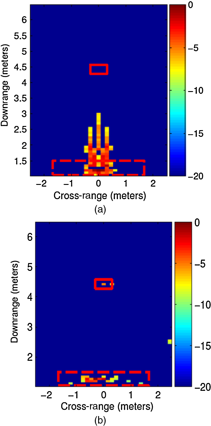

First, we consider the case when the same set of reduced frequencies is used for a reduced set of antenna locations. We employ only 10.2% of the data volume, i.e., 20% of the available frequencies and 51% of the antenna locations. The subspace projection method is applied to a $Y$ matrix of reduced dimension $146 \times 34$ . The corresponding $l_{1}$ norm reconstructed image obtained with OMP is depicted in Fig. 3(b). It is clear that, even when both spatial and frequency observations are reduced, the joint application of wall clutter mitigation and CS techniques successfully provides front wall clutter suppression and unmasking of the target.

4. Designated Dictionary for Wall Detection

In this section, we address the problem of imaging building interior structures using a reduced set of measurements. We consider interior walls as targets of interest and attempt to reveal the building interior layout based on CS techniques. We note that construction practices suggest the exterior and interior walls to be parallel or perpendicular to each other. This enables sparse scene representations using a dictionary of possible wall orientations and locations.⁷⁶ Conventional CS recovery algorithms can then be applied to reduced number of observations to recover the positions of various walls, which is a primary goal in TWRI.

4.1.

Signal Model Under Multiple Parallel Walls

Considering a monostatic stepped-frequency SAR system with $N$ antenna positions located parallel to the front wall, as shown in Fig. 1, we extend the signal model in Eq. (12) to include reflections from multiple parallel interior walls, in addition to the returns from the front wall and the $P$ point targets. That is, the received signal at the $n$ ’th antenna location corresponding to the $m$ ’th frequency can be expressed as

Eq. (21)

y (m, n) = σ_{w} \exp (- j ω_{m} τ_{w}) + \sum_{p = 0}^{P - 1} σ_{p} \exp (- j ω_{m} τ_{p, n}) + \sum_{i = 0}^{I_{w} - 1} σ_{w_{i}} \exp (- j ω_{m} τ_{w_{i}}),

where

I_{w}

is the number of interior walls parallel to the array axis,

τ_{w_{i}}

represents the two-way traveling time of the signal from the

n

’th antenna to the

i

’th interior wall and

σ_{w_{i}}

is the complex reflectivity of the

i

’th interior wall. Similar to the front wall, the delays

τ_{w_{i}}

are independent of the variable

n

, as evident in the subscripts.

Note that the above model contains contributions only from interior walls parallel to the front wall and the antenna array. This is because, due to the specular nature of the wall reflections, a SAR system located parallel to the front wall will only be able to receive direct returns from walls, which are parallel to the front wall. The detection of perpendicular walls is possible by concurrently detecting and locating the canonical scattering mechanism of corner features created by the junction of walls of a room or by having access to another side of the building. Extension of the signal model to incorporate corner returns is reported in Ref. 76.

Instead of the point-target based sensing matrix described in Eq. (7), where each antenna accumulates the contributions of all the pixels, we use an alternate sensing matrix, proposed in Ref. 68, to relate the scene vector, $r$ , and the observation vector, $y$ . This matrix underlines the specular reflections produced by the walls. Due to wall specular reflections, and since the array is assumed parallel to the front wall and, thus, parallel to interior walls, the rays collected at the $n$ ’th antenna will be produced by portions of the walls that are only in front of this antenna [see Fig. 4(a)]. The alternate matrix, therefore, only considers the contributions of the pixels that are located in front of each antenna. In so doing, the returns of the walls located parallel to the array axis are emphasized. As such, it is most suited to the specific building structure imaging problem, wherein the signal returns are mainly caused by EM reflections of exterior and interior walls. The alternate linear model can be expressed as

Eq. (22)

y = \bar{Ψ} r,

where

Eq. (23)

\bar{Ψ} = [\begin{matrix} {\bar{Ψ}}_{0}^{T} & {\bar{Ψ}}_{1}^{T} & \dots & {\bar{Ψ}}_{N - 1}^{T} \end{matrix}],

with

{\bar{Ψ}}_{n}

defined as

Eq. (24)

{[{\bar{Ψ}}_{n}]}_{m} = [\begin{matrix} I_{[(0, 0), n]} e^{- j ω_{m} τ_{(0, 0)}} & \dots & I_{[(N_{x} - 1, N_{z} - 1), n]} e^{- j ω_{m} τ_{(N_{x} - 1, N_{z} - 1)}} \end{matrix}] .

In Eq. (24),

τ_{k, l}

is the two-way signal propagation time associated with the downrange of the

(k, l)

’th pixel, and the function

I_{[(k, l), n]}

works as an indicator function in the following way:

Eq. (25)

I_{[(k, l), n]} = {\begin{matrix} 1, & if the {(k, l)}^{'} th pixel is in front of the n^{'} th antenna \\ 0, & otherwise \end{matrix} .

That is, if

x_{k}

and

x_{n}

represent the cross-range coordinates of the

(k, l)

’th pixel and the

n

’th antenna location, respectively, and

\partial x

is the cross-range sampling step, then

I_{[(k, l), n]} = 1

provided that

x_{k} - \partial x / 2 \leq x_{n} \leq x_{k} + \partial x / 2

[see Fig. 4(b)].

Fig. 4

(a) Specular reflections produced by walls; (b) indicator function.

4.2.

Sparsifying Dictionary for Wall Detection

Since the number of parallel walls is typically much smaller compared with the downrange extent of the building, the decomposition of the image into parallel walls can be considered as sparse. Note that although other indoor targets, such as furniture and humans, may be present, their projections onto the horizontal lines are expected to be negligible compared to those of the walls.

In order to obtain a linear matrix-vector relation between the scene and the horizontal projections, we define a sparsifying matrix $R$ composed of possible wall locations. Specifically, each column of the dictionary $R$ represents an image containing a single wall of length $l_{x}$ pixels, located at a specific cross-range and at a specific downrange in the image. Consider the cross-range to be divided into $N_{c}$ nonoverlapping blocks of $l_{x}$ pixels each [see Fig. 5(a)], and the downrange division defined by the pixel grid. The number of blocks $N_{c}$ is determined by the value of $l_{x}$ , which is the minimum expected wall length in the scene. Therefore, the dimension of $R$ is $N_{x} N_{z} \times N_{c} N_{z}$ ,where the product $N_{c} N_{z}$ denotes the number of possible wall locations. Figure 5(b) shows a simplified scheme of the sparsifying dictionary generation. The projection associated with each wall location is given by

Eq. (26)

g^{(b)} (l) = \frac{1}{l_{x}} \sum_{k \in B [b]} r (k, l),

where

B [b]

indicates the

b

’th cross-range block and

b = 1, 2, \dots, N_{c}

. Defining

Eq. (27)

g = [\begin{matrix} g^{(1)} (0) & \dots & g^{(N_{c})} (0) & g^{(1)} (1) & \dots & g^{(N_{c})} (1) & \dots & g^{(1)} (N_{z} - 1) & \dots & g^{(N_{c})} (N_{z} - 1) \end{matrix}],

the linear system of equations relating the observed data

y

and the sparse vector

g

is given by

Eq. (28)

y = \bar{Ψ} R g .

In practice and by the virtue of collecting signal reflections corresponding to the zero aspect angle, any interior wall outside the synthetic array extent will not be visible to the system. Finally, the CS image in this case is obtained by first recovering the projection vector

g

using

l_{1}

norm minimization with a reduced set of measurements and then forming the product

R g

.

Fig. 5

(a) Cross-range division into blocks of $l_{x}$ pixels; (b) Sparsifying dictionary generation.

It is noted that we are implicitly assuming that the extents of the walls in the scene are integer multiples of the block of $l_{x}$ pixels. In case this condition is not satisfied, the maximum error in determining the wall extent will be at most equal to the chosen block size. Note that incorporation of the corner effects will help resolve this issue, since the localization of corners will identify the wall extent.⁷⁶

4.3.

Illustrative Results

A through-the-wall SAR system was set up in the Radar Imaging Lab, Villanova University. A stepped-frequency signal consisting of 335 frequencies covering the 1 to 2 GHz frequency band was used for interrogating the scene. A monostatic synthetic aperture array, consisting of 71-element locations with an inter-element spacing of 2.2 cm, was employed. The scene consisted of two parallel plywood walls, each 2.25 cm thick, 1.83 m wide, and 2.43 m high. Both walls were centered at 0 m in cross-range. The first and the second walls were located at respective distances of 3.25 and 5.1 m from the antenna baseline. Figure 6(a) depicts the geometry of the experimental scene.

Fig. 6

(a) Scene geometry; (b) reconstructed image.

The region to be imaged is chosen to be $5.65 (cross - range) \times 4.45 m (down range)$ , centered at (0, 4.23) m, and is divided into $128 \times 128 pixels$ . For the CS approach, we use a uniform subset of only 84 frequencies at each of the 18 uniformly spaced antenna locations, which represent 6.4% of the full data volume. The CS reconstructed image is shown in Fig. 6(b). We note that the proposed algorithm was able to reconstruct both walls. However, it can be observed in Fig. 6(b) that ghost walls appear immediately behind each true wall position. These ghosts are attributed to the dihedral-type reflections from the wall-floor junctions.

5. CS and Multipath Exploitation

In this section, we consider the problem of multipath in view of the requirements of fast data acquisition and reduced measurements. Multipath ghosts may cast a sparse scene as a populated scene, and at minimum will render the scene less sparse, degrading the performance of CS-based reconstruction. A CS method that directly incorporates multipath exploitation into sparse signal reconstruction for imaging of stationary scenes with a stepped-frequency monostatic SAR is presented. Assuming prior knowledge of the building layout, the propagation delays corresponding to different multipath returns for each assumed target position are calculated, and the multipath returns associated with reflections from the same wall are grouped together and represented by one measurement matrix. This allows CS solutions to focus the returns on the true target positions without ghosting. Although not considered in this section, it is noted that the clutter due to front wall reverberations can be mitigated by adapting a similar multipath formulation, which maps back multiple reflections within the wall after separating wall and target returns.¹⁰⁰

5.1.

Multipath Propagation Model

We refer to the signal that propagates from the antenna through the front wall to the target and back to the antenna as the direct target return. Multipath propagation corresponds with indirect paths, which involve reflections at one or more interior walls by which the signal may reach the target. Multipath can also occur due to reflections from the floor and ceiling and interactions among different targets. In considering wall reflections and assuming diffuse target scattering, there are two typical cases for multipath. In the first case, the wave traverses a path that consists of two parts—one part is the propagation path to the target and back to the receiver, and the other part is a round trip path from the target to an interior wall. As the signal weakens at each secondary wall reflection, this case can usually be neglected. Furthermore, except when the target is close to an interior wall, the corresponding propagation delay is high and, most likely, would be equivalent to the direct-path delay of a target that lies outside the perimeter of the room being imaged. Thus, if necessary, this type of multipath can be gated out. The second case is a bistatic scattering scenario, where the signal propagation on transmit and receive takes place along different paths. This is the dominant case of multipath with one of the paths being the direct propagation, to or from the target, and the other involving a secondary reflection at an interior wall.

Other higher-order multipath returns are possible as well. Signals reaching the target can undergo multiple reflections within the front wall. We refer to such signals as wall ringing multipaths. Also the reflection at the interior wall can occur at the outer wall-air interface. This will result, however, in additional attenuation and, therefore, can be neglected. In order to derive the multipath signal model, we assume perfect knowledge of the front wall, i.e., location, thickness, and dielectric constant, as well as the location of the interior walls.

5.1.1.

Interior wall multipath

Consider the antenna-target geometry illustrated in Fig. 7(a), where the front wall has been ignored for simplicity. The $p$ ’th target is located at $x_{p} = (x_{p}, z_{p})$ , and the interior wall is parallel to the $z$ -axis and located at $x = x_{w}$ . Multipath propagation consists of the forward propagation from the $n$ ’th antenna to the target along the path $P^{''}$ and the return from the target via a reflection at the interior wall along the path $P^{'}$ . Assuming specular reflection at the wall interface, we observe from Fig. 7(a) that reflecting the return path about the interior wall yields an alternative antenna-target geometry. We obtain a virtual target located at ${x^{'}}_{p} = (2 x_{w} - x_{p}, z_{p})$ , and the delay associated with path $P^{'}$ is the same as that of the path ${\tilde{P}}^{'}$ from the virtual target to the antenna. This correspondence simplifies the calculation of the one-way propagation delay $τ_{p, n}^{(P'})$ associated with path $P^{'}$ . It is noted that this principle can be used for multipath via any interior wall.

Fig. 7

(a) Multipath propagation via reflection at an interior wall; (b) wall ringing propagation with $i_{w} = 1$ internal bounces.

From the position of the virtual target of an assumed target location, we can calculate the propagation delay along path $P^{'}$ as follows. Under the assumption of free space propagation, the delay can be simply calculated as the Euclidean distance from the virtual target to the receiver divided by the propagation speed of the wave. In the TWRI scenario, however, the wave has to pass through the front wall on its way from the virtual target to the receiver. As the front wall parameters are assumed to be known, the delay can be readily calculated from geometric considerations using Snell’s law.²⁸

5.1.2.

Wall ringing multipath

The effect of wall ringing on the target image can be delineated through Fig. 7(b), which depicts the wall and the incident, reflected, and refracted waves. The distance between the target and the array element in cross-range direction, $Δ x$ , can be expressed as

Eq. (29)

Δ x = (Δ z - d) \tan θ_{air} + d (1 + 2 i_{w}) \tan θ_{wall},

where

Δ z

is the distance between target and array element in downrange direction, and

θ_{air}

and

θ_{wall}

are the angles in the air and in the wall medium, respectively. The integer

i_{w}

denotes the number of internal reflections within the wall. The case

i_{w}

=0 describes the direct path as derived in Ref. 28. From Snell’s law,

Eq. (30)

\frac{\sin θ_{air}}{\sin θ_{wall}} = \sqrt{ε} .

Equations (29) and (30) form a nonlinear system of equations that can be solved numerically for the unknown angles, e.g., using the Newton method. Having the solution for the incidence and refraction angles, we can express the one-way propagation delay associated with the wall ringing multipath as¹⁰¹

Eq. (31)

τ = \frac{(Δ z - d)}{c \cos θ_{air}} + \frac{\sqrt{ε} d (1 + 2 i_{w})}{c \cos θ_{wall}} .

5.2.

Received Signal Model

Having described the two principal multipath mechanisms in TWRI, namely the interior wall and wall ringing types of multipath, we are now in a position to develop a multipath model for the received signal. We assume that the front wall returns have been suppressed and the measured data contains only the target returns. The case with the wall returns present in the measurements is discussed in Ref. 100.

Each path $P$ from the transmitter to a target and back to receiver can be divided into two parts, $P^{'}$ and $P^{''},$ where $P^{''}$ denotes the partial path from the transmitter to the scattering target and $P^{'}$ is the return path back to the receiver. For each target-transceiver combination, there exist a number of partial paths due to the interior wall and wall ringing multipath phenomena. Let $P_{i_{1}}^{'}$ , $i_{1} = 0, 1, \dots, R_{1} - 1$ , and $P_{i_{2}}^{''}$ , $i_{2} = 0, 1, \dots, R_{2} - 1$ , denote the feasible partial paths. Any combination of $P_{i_{1}}^{'}$ and $P_{i_{2}}^{''}$ results in a round-trip path $P_{i}$ , $i = 0, 1, \dots, R - 1$ . We can establish a function that maps the index $i$ of the round-trip path to a pair of indices of the partial paths, $i \mapsto (i_{1}, i_{2})$ . Hence we can determine the maximum number $R \leq R_{1} R_{2}$ of possible paths for each target-transceiver pair. Note that, in practice, $R ≪ R_{1} R_{2}$ , as some round-trip paths may be equal due to symmetry while some others could be strongly attenuated and thereby can be neglected. We follow the convention that $P_{0}$ refers to the direct round-trip path.

The round-trip delay of the signal along path $P_{i}$ , consisting of the partial parts $P_{i_{1}}^{'}$ and $P_{i_{2}}^{''}$ ,can be calculated as

Eq. (32)

τ_{p, n}^{(i)} = τ_{p, n}^{(i_{1})} + τ_{p, n}^{(i_{2})} .

We also associate a complex amplitude

w_{p}^{(i)}

for each possible path corresponding to the

p

’th target, with the direct path, which is typically the strongest in TWRI, having

w_{p}^{(0)} = 1

.

Without loss of generality, we assume the same number of propagation paths for each target. The unavailability of a path for a particular target is reflected by a corresponding path amplitude of zero. The received signal at the $n$ ’th antenna due to the $m$ ’th frequency can, therefore, be expressed as

Eq. (33)

y (m, n) = \sum_{i = 0}^{R - 1} \sum_{p = 0}^{P - 1} w_{p}^{(i)} σ_{p}^{(i)} \exp (- j ω_{m} τ_{p, n}^{(i)}) .

As the bistatic radar cross-section (RCS) of a target could be different from its monostatic RCS, the target reflectivity is considered to be dependent on the propagation path. For convenience, the path amplitude

w_{p}^{(i)}

in Eq. (33) can be absorbed into the target reflectivity

σ_{p}^{(i)}

, leading to

Eq. (34)

y (m, n) = \sum_{i = 0}^{R - 1} \sum_{p = 0}^{P - 1} σ_{p}^{(i)} \exp (- j ω_{m} τ_{p, n}^{(i)}) .

Note that Eq. (34) is a generalization of the non-multipath propagation model in Eq. (2). If the number of propagation paths is set to 1, then the two models are equivalent.

The matrix-vector form for the received signal under multipath propagation is given by

Eq. (35)

y = Ψ^{(0)} r^{(0)} + Ψ^{(1)} r^{(1)} + \dots + Ψ^{(R - 1)} r^{(R - 1)},

where

Eq. (36)

r^{(i)} = {[\begin{matrix} r_{00}^{(i)} & \dots & r_{N_{x} N_{z} - 1}^{(i)} \end{matrix}]}^{\begin{array}{l} T \end{array}} {[Ψ^{(i)}]}_{s q} = \exp (- j ω_{m} τ_{q, n}^{(i)}), m = s \mod M, n = ⌊ s / M ⌋ s = 0, 1, \dots, M N - 1, q = 0, 1, \dots, N_{x} N_{z} - 1 .

The term

r_{q}^{(i)}

,

q = 0, 1, \dots, N_{x} N_{z} - 1

, takes the value

σ_{p}^{(i)}

if the

p

’th point target exists at the

q

’th pixel; otherwise, it is zero. Finally, the reduced measurement vector

\overset{̆}{y}

can be obtained from Eq. (35) as

\overset{̆}{y} = Φ y

, where the

Q_{1} Q_{2} \times M N

matrix

Φ

is defined in Eq. (10).

5.3.

Sparse Scene Reconstruction with Multipath Exploitation

Within the CS framework, we aim at undoing the ghosts, i.e., inverting the multipath measurement model and achieving a reconstruction, wherein only the true targets remain.

In practice, any prior knowledge about the exact relationship between the various subimages $r^{(i)}$ of the sparse scene is either limited or nonexistent. However, we know with certainty that the sub-images $r^{(0)}, r^{(1)}, \dots r^{(R - 1)}$ describe the same underlying scene. That is, the support of the $R$ images is the same, or at least approximately the same. The common structure property of the sparse scene suggests the application of a group sparse reconstruction.

All unknown vectors in Eq. (35) can be stacked to form a tall vector of length $N_{x} N_{z} R$

Eq. (37)

\vec{r} = {[\begin{matrix} r^{{(0)}^{T}} & r^{{(1)}^{T}} & \dots & r^{{(R - 1)}^{T}} \end{matrix}]}^{T} .

The reduced measurement vector

\overset{̆}{y}

can then be expressed as

Eq. (38)

\overset{̆}{y} = B \vec{r},

where

B = ⌊ \begin{matrix} Φ Ψ^{(0)} & Φ Ψ^{(1)} & \dots & Φ Ψ^{(R - 1)} \end{matrix} ⌋

has dimensions

Q_{1} Q_{2} \times N_{x} N_{z} R

.

We proceed to reconstruct the images $\vec{r}$ from $\overset{̆}{y}$ under measurement model in Eq. (38). It has been shown that a group sparse reconstruction can be obtained by a mixed $l_{1} - l_{2}$ norm regularization.¹⁰²^–¹⁰⁵ Thus we solve

Eq. (39)

\hat{\vec{r}} = \arg \min_{\vec{r}} \frac{1}{2} ‖ \overset{̆}{y} - B \vec{r} ‖ + α {‖ \vec{r} ‖}_{2, 1},

where

α

is the so-called regularization parameter and

Eq. (40)

{‖ \vec{r} ‖}_{2, 1} = \sum_{q = 0}^{N_{x} N_{z} - 1} {‖ {[r_{q}^{(0)}, r_{q}^{(1)}, \dots, r_{q}^{(R - 1)}]}^{T} ‖}_{2} = \sum_{q = 0}^{N_{x} N_{z} - 1} \sqrt{\sum_{i = 0}^{R - 1} r_{q}^{(i)} r_{q}^{{(i)}^{*}}}

is the mixed

l_{1} - l_{2}

norm. As defined in Eq. (40), the mixed

l_{1} - l_{2}

norm behaves like an

l_{1}

norm on the vector

{‖ {[r_{q}^{(0)}, r_{q}^{(1)}, \dots, r_{q}^{(R - 1)}]}^{T} ‖}_{2}

q = 0, 1, \dots, N_{x} N_{z} - 1

, and therefore induces group sparsity. In other words, each

{‖ {[r_{q}^{(0)}, r_{q}^{(1)}, \dots, r_{q}^{(R - 1)}]}^{T} ‖}_{2}

, and equivalently each

{[r_{q}^{(0)}, r_{q}^{(1)}, \dots, r_{q}^{(R - 1)}]}^{T}

, are encouraged to be set to zero. On the other hand, within the groups, the

l_{2}

norm does not promote sparsity.¹⁰⁶ The convex optimization problem in Eq. (39) can be solved using SparSA,¹⁰² YALL group,¹⁰³ or other available schemes.¹⁰⁵^,¹⁰⁷

Once a solution $\hat{\vec{r}}$ is obtained, the subimages can be noncoherently combined to form an overall image with an improved signal-to-noise-and-clutter ratio (SCNR), with the elements of the composite image ${\hat{r}}_{GS}$ defined as

Eq. (41)

{[{\hat{r}}_{GS}]}_{q} = {‖ {[r_{q}^{(0)}, r_{q}^{(1)}, \dots, r_{q}^{(R - 1)}]}^{T} ‖}_{2}, q = 0, \dots, N_{x} N_{z} - 1 .

5.4.

Illustrative Results

An experiment was conducted in a semi-controlled environment at the Radar Imaging Lab, Villanova University. A single aluminum pipe (61 cm long, 7.6 cm diameter) was placed upright on a 1.2-m-high foam pedestal at 3.67 m downrange and 0.31 m cross-range, as shown in Fig. 8. A 77-element uniform linear monostatic array with an inter-element spacing of 1.9 cm was used for imaging. The origin of the coordinate system is chosen to be at the center of the array. The 0.2-m-thick concrete front wall was located parallel to the array at 2.44 m downrange. The left sidewall was at a cross-range of $- 1.83 m$ , whereas the back wall was at 6.37 m downrange (see Fig. 8). Also there was a protruding corner on the right at 3.4 m cross-range and 4.57 m downrange. A stepped-frequency signal, consisting of 801 equally spaced frequency steps covering the 1 to 3 GHz band was employed. The left and right side walls were covered with RF absorbing material, but the protruding right corner and the back wall were left uncovered.

Fig. 8

Scene layout.

We consider background-subtracted data to focus only on target multipath. Figure 9(a) depicts the backprojection image using all available data. Apparently, only the multipath ghosts due to the back wall, and the protruding corner in the back right are visible. Hence we only consider these two multipath propagation cases for the group sparse CS scheme. We use 25% of the array elements and 50% of the frequencies. The corresponding CS reconstruction is shown in Fig. 9(b). The multipath ghosts have been clearly suppressed.

Fig. 9

(a) Back-projection image with full data volume; (b) group sparse reconstruction with 25% of the antenna elements and 50% of the frequencies.

6. CS-Based Change Detection for Moving Target Localization

In this section, we consider sparsity-driven CD for human motion indication in TWRI applications. CD can be used in lieu of Doppler processing, wherein motion detection is accomplished by subtraction of data frames acquired over successive probing of the scene. In so doing, CD mitigates the heavy clutter that is caused by strong reflections from exterior and interior walls and also removes stationary objects present in the enclosed structure, thereby rendering a densely populated scene sparse.⁷^,⁹^,¹⁰ As a result, it becomes possible to exploit CS techniques for achieving reduction in the data volume. We assume a multistatic imaging system with physical transmit and receive apertures and a wideband transmit pulse. We establish an appropriate CD model for translational motion that permits formulation of linear modeling with sensing matrices, so as to apply CS for scene reconstruction. Other types of human motions involving sudden short movements of the limbs, head, and/or torso are discussed in Ref. 70.

6.1.

Signal Model

Consider wideband radar operation with $M$ transmitters and $N$ receivers. A sequential multiplexing of the transmitters with simultaneous reception at multiple receivers is assumed. As such, a signal model can be developed based on single active transmitters. We note that the timing interval for each data frame is assumed to be a fraction of a second so that the moving target appears stationary during each data collection interval.

Let $s_{T} (t)$ be the wideband baseband signal used for interrogating the scene. For the case of a single point target with reflectivity $σ_{p}$ , located at $x_{p} = (x_{p}, z_{p})$ behind a wall, the pulse emitted by the $m$ ’th transmitter with phase center at $x_{tm} = (x_{tm}, - z_{off})$ is received at the $n$ ’th receiver with phase center at $x_{rn} = (x_{rn}, - z_{off})$ in the form

Eq. (42)

y_{m n} (t) = a_{m n} (t) + b_{m n} (t), a_{m n} (t) = σ_{p} s_{T} (t - τ_{p, m n}) \exp (- j ω_{c} τ_{p, m n}),

where

ω_{c}

is the carrier frequency,

τ_{p, m n}

is the propagation delay for the signal to travel between the

m

’th transmitter, the target at

x_{p}

, and the

n

’th receiver, and

b_{m n} (t)

represents the contribution of the stationary background at the

n

’th receiver with the

m

’th transmitter active. The delay

τ_{p, m n}

consists of the components corresponding to traveling distances before, through, and after the wall, similar to Eq. (3).

In its simplest form, CD is achieved by coherent subtraction of the data corresponding to two data frames, which may be consecutive or separated by one or more data frames. This subtraction operation is performed for each range bin. CD results in the set of difference signals,

Eq. (43)

δ y_{m n} (t) = y_{m n}^{(L + 1)} (t) - y_{m n}^{(1)} (t) = a_{m n}^{(L + 1)} (t) - a_{m n}^{(1)} (t),

where

L

denotes the number of frames between the two time acquisitions. The component of the radar return from the stationary background is the same over the two time intervals and is thus removed from the difference signal. Using Eqs. (42) and (43), the

(m, n)

’th difference signal can be expressed as

Eq. (44)

δ y_{m n} (t) = σ_{p} s_{T} (t - τ_{p, m n}^{(L + 1)}) \exp (- j ω_{c} τ_{p, m n}^{(L + 1)}) - σ_{p} s_{T} (t - τ_{p, m n}^{(1)}) \exp (- j ω_{c} τ_{p, m n}^{(1)}),

where

τ_{p, m n}^{(1)}

and

τ_{p, m n}^{(L + 1)}

are the respective two-way propagation delays for the signal to travel between the

m

’th transmitter, the target, and the

n

’th receiver, during the first and the second data acquisitions, respectively.

6.2.

Sparsity-Driven Change Detection under Translational Motion

Consider the difference signal in Eq. (44) for the case where the target is undergoing translational motion. Two nonconsecutive data frames with relatively long time difference are used, i.e., $L ≫ 1$ (Ref. 108). In this case, the target will change its range gate position during the time elapsed between the two data acquisitions. As seen from Eq. (44), the moving target will present itself as two targets, one corresponding to the target position during the first time interval, and the other corresponding to the target location during the second data frame. It is noted that the imaged target at the reference position corresponding to the first data frame cannot be suppressed for the coherent CD approach. On the other hand, the noncoherent CD approach that deals with differences of image magnitudes corresponding to the two data frames, allows suppression of the reference image through a zero-thresholding operation.²³ However, as the noncoherent approach requires the scene reconstruction to be performed prior to CD, it is not a feasible option for sparsity-based imaging, which relies on coherent CD to render the scene sparse. Therefore, we rewrite Eq. (44) as

Eq. (45)

δ y_{m n} (t) = \sum_{i = 1}^{2} {\tilde{σ}}_{i} s_{T} (t - τ_{i, m n}) \exp (- j ω_{c} τ_{i, m n}),

with

Eq. (46)

{\tilde{σ}}_{i} = {\begin{matrix} σ_{p} & i = 1 \\ - σ_{p} & i = 2 \end{matrix} and τ_{i, m n} = {\begin{matrix} τ_{p, m n}^{(L + 1)} & i = 1 \\ τ_{p, m n}^{(1)} & i = 2 \end{matrix} .

If we sample the difference signal

δ y_{m n} (t)

at times

{t_{k}}_{k = 0}^{K - 1}

to obtain the

K \times 1

vector

{Δ y}_{m n}

and form the concatenated

N_{x} N_{z} \times 1

scene reflectivity vector

r

, then using the developed signal model in Eq. (45), we obtain the linear system of equations

Eq. (47)

{Δ y}_{m n} = Ψ_{m n} r .

The

q

’th column of

Ψ_{m n}

consists of the received signal corresponding to a target at pixel

x_{q}

and the

k

’th element of the

q

’th column can be written as⁷⁰^,⁸³

Eq. (48)

{[Ψ_{m n}]}_{k, q} = \frac{s_{T} (t_{k} - τ_{q, m n}) \exp (- j ω_{c} τ_{q, m n})}{{‖ s_{q, m n} ‖}_{2}}, k = 0, 1, \dots, K - 1, q = 0, 1, \dots, N_{x} N_{z} - 1,

where

τ_{q, m n}

is the two-way signal traveling time from the

m

’th transmitter to the

q

’th pixel and back to the

n

’th receiver. Note that the

k

’th element of the vector

s_{q, m n}

is

s_{T} (t_{k} - τ_{q, m n})

, which implies that the denominator in the R.H.S. of Eq. (48) is the energy in the time signal. Therefore, each column of

Ψ_{m n}

has unit norm. Further note that if there is a target at the

q

’th pixel, the value of the

q

’th element of

r

should be

{\tilde{σ}}_{q}

; otherwise, it is zero.

The CD model described in Eqs. (47) and (48) permits the scene reconstruction within the CS framework. We measure a $J (≪ K)$ dimensional vector of elements randomly chosen from ${Δ y}_{m n}$ . The new measurements can be expressed as

Eq. (49)

Δ {\overset{̆}{y}}_{m n} = φ_{m n} {Δ y}_{m n} = φ_{m n} Ψ_{m n} r,

where

φ_{m n}

is a

J \times K

measurement matrix. Several types of measurement matrices have been reported in the literature⁸³^,⁸⁶^,¹⁰⁹ and the references therein. To name a few, a measurement matrix whose elements are drawn from a Gaussian distribution, a measurement matrix having random

\pm 1

entries with probability of 0.5, or a random matrix whose entries can be constructed by randomly selecting rows of a

K \times K

identity matrix. It was shown in Ref. 83 that the measurement matrix with random

\pm 1

elements requires the least amount of compressive measurements for the same radar imaging performance, and permits a relatively straight forward data acquisition implementation. Therefore, we choose to use such a measurement matrix in image reconstructions.

Given $Δ {\overset{̆}{y}}_{m n}$ for $m = 0$ , $1, \dots, M - 1$ , $n = 0$ , $1, \dots, N - 1$ , we can recover $r$ by solving the following equation:

Eq. (50)

\hat{r} = \arg \min_{r} {‖ r ‖}_{l_{1}} subject to Φ Ψ r \approx Δ \overset{̆}{y},

where

Eq. (51)

Ψ = {[Ψ_{00}^{T} Ψ_{01}^{T} \dots Ψ_{(M - 1) (N - 1)}^{T}]}^{T}, Φ = diag (φ_{00}, φ_{01}, \dots, φ_{(M - 1) (N - 1)}) Δ \overset{̆}{y} = {[Δ {\overset{̆}{y}}_{00}^{T} Δ {\overset{̆}{y}}_{01}^{T} \dots Δ {\overset{̆}{y}}_{(M - 1) (N - 1)}^{T}]}^{T} .

Equations (50) and (51) represent one strategy that can be adopted for sparsity-based CD approach, wherein a reduced number of time samples are chosen randomly for all the transmitter-receiver pairs constituting the array apertures. The above two equations can also be extended so that the reduction in data measurements includes both spatial and time samples. The latter strategy is not considered in this section.

6.3.

Illustrative Results

A through-the-wall wideband pulsed radar system was used for data collection in the Radar Imaging Lab at Villanova University. The system uses a 0.7 ns Gaussian pulse for scene interrogation. The pulse is up-converted to 3 GHz for transmission and down-converted to baseband through in-phase and quadrature demodulation on reception. The system operational bandwidth from 1.5 to 4.5 GHz provides a range resolution of 5 cm. The peak transmit power is 25 dBm. Transmission is through a single horn antenna, which is mounted on a tripod. An eight-element line array with an inter-element spacing of 0.06 m, is used as the receiver and is placed to the right of the transmit antenna. The center-to-center separation between the transmitter and the leftmost receive antenna is 0.28 m, as shown in Fig. 10. A $3.65 \times 2.6 m^{2}$ wall segment was constructed utilizing 1-cm-thick cement board on a 2-x-4 wood stud frame. The transmit antenna and the receive array were at a standoff distance of 1.19 m from the wall. The system refresh rate is 100 Hz.

Fig. 10

Scene layout for the target undergoing translational motion.

In the experiment, a person walked away from the wall in an empty room (the back and the side walls were covered with RF absorbing material) along a straight line path. The path is located 0.5 m to the right of the center of the scene, as shown in Fig. 10. The data collection started with the target at position 1 and ended after the target reached position 3, with the target pausing at each position along the trajectory for a second. Consider the data frames corresponding to the target at positions 2 and 3. Each frame consists of 20 pulses, which are coherently integrated to improve the signal-to-noise ratio. The imaging region (target space) is chosen to be $3 \times 3 m^{2}$ , centered at (0.5 m, 4 m), and divided into $61 \times 61$ grid points in cross-range and downrange, resulting in 3721 unknowns. The space-time response of the target space consists of $8 \times 1536$ space-time measurements. For sparsity-based CD, only 5% of the 1536 time samples are randomly selected at each of the eight receive antenna locations, resulting in $8 \times 77$ space-time measured data. Figure 11 depicts the corresponding result. We observe that, as the human changed its range gate position during the time elapsed between the two acquisitions, it presents itself as two targets in the image, and is correctly localized at both of its positions.

Fig. 11

Sparsity-based CD image using 5% of the data volume.

7. CS General Formulation for Stationary and Moving Targets

As seen in the previous sections, the presence of the front wall renders the target detection problem very difficult and challenging and has an adverse effect on the scene reconstruction performance when employing CS. Different strategies have been devised for suppression of the wall clutter to enable target detection behind walls. Change detection enables detection and localization of moving targets. Clutter cancellation filtering provides another option.⁸⁷^,¹¹⁰ However, along with the wall clutter, both of these methods also suppress the returns from the stationary targets of interest in the scene, and as such, allow subsequent application of CS to recover only the moving targets. Wall clutter mitigation methods can be applied to remove the wall and enable joint detection of stationary and moving targets. However, these methods assume monostatic operation with the array located parallel to the front wall and exploit the strength and invariance of the wall return across the array under such a deployment for mitigating the wall return. As such, they may not perform as well under other situations.

For multistatic imaging radar systems using ultra-wideband (UWB) pulses, an alternate option is to employ time gating, in lieu of the aforementioned clutter cancellation methods. The compact temporal support of the signal renders time gating a viable option for suppressing the wall returns. This enhances the SCR and maintains the sparsity of the scene, thereby permitting the application of CS techniques for simultaneous localization of stationary and moving targets with few observations.⁷⁴

7.1.

Signal Model

Consider the scene layout depicted in Fig. 12. Note that although the $M$ -element transmit and $N$ -element receive arrays are assumed to be parallel to the front wall for notational simplicity, this is not a requirement. Let $T_{r}$ be the pulse repetition interval. Consider a coherent processing interval of $I$ pulses per transmitter and a single point target moving slowly away from the origin with constant horizontal and vertical velocity components $(v_{x p}, v_{z p})$ , as depicted in Fig. 12. Let the target position be $x_{p} = (x_{p}, z_{p})$ at time $t = 0$ . Assume that the timing interval for sequencing through the transmitters is short enough so that the target appears stationary during each data collection interval of length ${IT}_{r}$ . This implies that the target position corresponding to the $i$ ’th pulse is given by

Eq. (52)

x_{p} (i) = (x_{p} + v_{x p} i I T_{r}, z_{p} + v_{z p} i I T_{r}) .

The baseband target return measured by the

n

’th receiver corresponding to the

i ’ th

pulse emitted by the

m

’th transmitter is given by⁷⁴

Eq. (53)

y_{m n i}^{p} (t) = σ_{p} s_{T} [t - i {IT}_{r} - m T_{r} - τ_{p, m n} (i)] \exp [- j ω_{c} τ_{p, m n} (i)],

where

τ_{p, m n} (i)

is the propagation delay for the

i

’th pulse to travel from the

m

’th transmitter to the target at

x_{p} (i)

, and back to the

n

’th receiver. In the presence of

P

point targets, the received signal component corresponding to the targets will be a superposition of the individual target returns in (53) with

p = 0, 1, \dots, P - 1

. Interactions between the targets and multipath returns are ignored in this model. Note that any stationary targets behind the wall are included in this model and would correspond to the motion parameter pair

(v_{x p}, v_{z p}) = (0, 0)

. Further note that the slowly moving targets are assumed to remain within the same range cell over the coherent processing interval.

Fig. 12

Geometry on transmit and receive.

On the other hand, as the wall is a specular reflector, the baseband wall return received at the $n$ ’th receiver corresponding to the $i$ ’th pulse emitted by the $m$ ’th transmitter can be expressed as

Eq. (54)

y_{m n i}^{wall} (t) = σ_{w} s_{T} [t - i {IT}_{r} - m T_{r} - τ_{w, m n})] \exp (- j ω_{c} τ_{w, m n}) + B_{m n i}^{wall} (t),

where

τ_{w, m n}

is the propagation delay from the

m

’th transmitter to the wall and back to the

n

’th receiver, and

B_{m n i}^{wall} (t)

represents the wall reverberations of decaying amplitudes resulting from multiple reflections within the wall (see Fig. 13). The propagation delay

τ_{w, m n}

is given by¹¹¹

Eq. (55)

τ_{w, m n} = \frac{\sqrt{{(x_{tm} - x_{w, m n})}^{2} + z_{off}^{2}} + \sqrt{{(x_{r n} - x_{w, m n})}^{2} + z_{off}^{2}}}{c},

where

Eq. (56)

x_{w, m n} = \frac{x_{tm} + x_{rn}}{2},

is the point of reflection on the wall corresponding to the

m

’th transmitter and the

n

’th receiver, as shown in Fig. 13. Note that, as the wall is stationary, the delay

τ_{w, m n}

does not vary from one pulse to the next. Therefore the expression in Eq. (54) assumes the same value for

i = 0, 1, \dots, I - 1

.

Fig. 13

Wall reverberations.

Combining Eqs. (53) and (54), the total baseband signal received by the $n$ ’th receiver, corresponding to the $i$ ’th pulse with the $m$ ’th transmitter active, is given by

Eq. (57)

y_{m n i}^{'} (t) = y_{m n i}^{wall} (t) + \sum_{p = 0}^{P - 1} y_{m n i}^{p} (t) .

By gating out the wall return in the time domain, we gain access to the sparse behind-the-wall scene of a few stationary and moving targets of interest. Therefore the time-gated received signal contains only contributions from the $P$ targets behind the wall as well as any residuals of the wall not removed or fully mitigated by gating. In this section, we assume that wall clutter is effectively suppressed by gating. Therefore, using Eq. (57), we obtain

Eq. (58)

y_{m n i} (t) = \sum_{p = 0}^{P - 1} y_{m n i}^{p} (t) .

7.2.

Linear Model Formulation and CS Reconstruction

With the observed scene divided into $N_{x} \times N_{z}$ pixels in cross-range and downrange, consider $N_{v_{x}}$ and $N_{v_{z}}$ discrete values of the expected horizontal and vertical velocities, respectively. Therefore an image with $N_{x} \times N_{z}$ pixels in cross-range and downrange is associated with each considered horizontal and vertical velocity pair, resulting in a four-dimensional (4-D) target space. Note that the considered velocities contain the (0, 0) velocity pair to include stationary targets.

Sampling the received signal $y_{m n i} (t)$ at times ${t_{k}}_{k = 0}^{K - 1}$ , we obtain a $K \times 1$ vector $y_{m n i}$ . For the $l$ ’th velocity pair $(v_{x l}, v_{z l})$ , we vectorize the corresponding cross-range versus downrange image into an $N_{x} N_{z} \times 1$ scene reflectivity vector $r (v_{x l}, v_{z l})$ . The vector $r (v_{x l}, v_{z l})$ is a weighted indicator vector defining the scene reflectivity corresponding to the $l$ ’th considered velocity pair, i.e., if there is a target at the spatial grid point ( $x$ , $z$ ) with motion parameters $(v_{x l}, v_{z l})$ , then the value of the corresponding element of $r (v_{x l}, v_{z l})$ should be nonzero; otherwise, it is zero.

Using the developed signal model in Eqs. (53) and (58), we obtain the linear system of equations

Eq. (59)

y_{m n i} = Ψ_{m n i} (v_{x l}, v_{z l}) r (v_{x l}, v_{z l}), l = 0, 1, \dots, N_{v_{x}} N_{v_{z}} - 1,

where the matrix

Ψ_{m n i} (v_{x l}, v_{z l})

is of dimension

K \times N_{x} N_{z}

. The

q

’th column of

Ψ_{m n i} (v_{x l}, v_{z l})

consists of the received signal corresponding to a target at pixel

x_{q}

with motion parameters

(v_{x l}, v_{z l})

, and the

i

’th element of the

q

’th column can be written as

Eq. (60)

{[Ψ_{m n i} (v_{x l}, v_{z l})]}_{k, q} = s_{T} [t_{k} - i I T_{r} - m T_{r} - τ_{q, m n} (i)] \exp [- j ω_{c} τ_{q, m n} (i)], q = 0, 1, \dots, N_{x} N_{z} - 1

where

τ_{q, m n} (i)

is the two-way signal traveling time, corresponding to

(v_{x l}, v_{z l})

, from the

m

’th transmitter to the

q

’th spatial grid point and back to the

n

’th receiver for the

i

’th pulse.

Stacking the received signal samples corresponding to $I$ pulses from all $M N$ transmitting and receiving element pairs, we obtain the $M N I K \times 1$ measurement vector $y$ as

Eq. (61)

y = Ψ (v_{x l}, v_{z l}) r (v_{x l}, v_{z l}), l = 0, 1, \dots, (N_{v_{x}} N_{v_{z}} - 1),

where

Eq. (62)

Ψ (v_{x l}, v_{z l}) = {[Ψ_{000}^{T} (v_{x l}, v_{z l}), \dots, Ψ_{(M - 1) (N - 1) (I - 1)}^{T} (v_{x l}, v_{z l})]}^{T} .

Finally, forming the

M N I K \times N_{x} N_{z} N_{v_{x}} N_{v_{z}}

matrix

Ψ

as

Eq. (63)

Ψ = [Ψ (v_{x 0}, v_{z 0}), \dots, Ψ (v_{x (N_{v_{x}} N_{v_{z}} - 1)}, v_{z (N_{v_{x}} N_{v_{z}} - 1)})],

we obtain the linear matrix equation

Eq. (64)

y = Ψ \hat{r},

with

\hat{r}

being the concatenation of target reflectivity vectors corresponding to every possible considered velocity combination.

The model described in Eq. (64) permits the scene reconstruction within the CS framework. We measure a $J < M N I K$ dimensional vector of elements randomly chosen from $y$ . The reduced set of measurements can be expressed as

Eq. (65)

\overset{̆}{y} = Φ Ψ \hat{r},

where

Φ

is a

J \times M N I K

measurement matrix. For measurement reduction simultaneously along the spatial, slow time, and fast time dimensions, the specific structure of the matrix

Φ

is given by

Eq. (66)

Φ = kron (Φ_{1}, I_{J_{1} J_{2} N_{1}}) \cdot kron (Φ_{2}, I_{J_{1} J_{2} M}) \cdot kron (Φ_{3}, I_{J_{1} M N}) \cdot diag {Φ_{4}^{(0)}, Φ_{4}^{(1)}, \dots, Φ_{4}^{(M N I - 1)}},

where

I_{(\cdot)}

is an identity matrix with the subscript indicating its dimensions, and

M_{1}, N_{1}, J_{1}

, and

J_{2}

denote the reduced number of transmit elements, receive elements, pulses, and fast time samples, respectively, with the total number of reduced measurements

J = M_{1} N_{1} J_{1} J_{2}

. The matrix

Φ_{1}

is an

M_{1} \times M

matrix,

Φ_{2}

is an

N_{1} \times N

matrix,

Φ_{3}

is a

J_{2} \times I

matrix, and each of the

Φ_{4}

matrices is a

J_{1} \times K

matrix for determining the reduced number of transmitting elements, receiving elements, pulses and fast time samples, respectively. Each of the three matrices

Φ_{1}

,

Φ_{2}

, and

Φ_{3}

consists of randomly selected rows of an identity matrix. These choices of reduced matrix dimensions amount to selection of subsets of existing available degrees of freedom offered by the fully deployed imaging system. Any other matrix structure does not yield to any hardware simplicity or saving in acquisition time. On the other hand, three different choices, discussed in Sec. 6.2, are available for compressive acquisition of each pulse in fast time.

Given the reduced measurement vector $\overset{̆}{y}$ in Eq. (65), we can recover $\hat{r}$ by solving the following equation,

Eq. (67)

\hat{\hat{r}} = \arg \min_{\hat{r}} {∥ \hat{r} ∥}_{l_{1}} subject to Φ Ψ \hat{r} \approx \overset{̆}{y} .

We note that the reconstructed vector can be rearranged into

N_{v_{x}} N_{v_{z}}

matrices of dimensions

N_{x} \times N_{z}

in order to depict the estimated target reflectivity for different vertical and horizontal velocity combinations. Note that (1) stationary targets will be localized for the (0,0) velocity pair, and (2) two targets located at the same spatial location but moving with different velocities will be distinguished and their corresponding reflectivity and motion parameters will be estimated.

7.3.

Illustrative Results

A real data collection experiment was conducted in the Radar Imaging Laboratory, Villanova University. The system and signal parameters are the same as described in Sec. 6.3. The origin of the coordinate system was chosen to be at the center of the receive array. The scene behind the wall consisted of one stationary target and one moving target, as shown in Fig. 14. A metal sphere of 0.3 m diameter, placed on a 1-m-high Styrofoam pedestal, was used as the stationary target. The pedestal was located 1.25 m behind the wall, centered at (0.49 m, 2.45 m). A person walked toward the front wall at a speed of $0.7 m / s$ approximately along a straight line path, which is located 0.2 m to the right of the transmitter. The back and the right side wall in the region behind the front wall were covered with RF absorbing material, whereas the 8-in.-thick concrete side-wall on the left and the floor were uncovered. A coherent processing interval of 15 pulses was selected.

Fig. 14

The configuration of the experiment.

The image region is chosen to be $4 \times 6 m^{2}$ , centered at ( $- 0.31 m$ , $3 m$ ), and divided into $41 \times 36 pixels$ in cross-range and downrange. As the human moves directly toward the radar, we only consider varying vertical velocity from $- 1.4$ to $0 m / s$ , with a step size of $0.7 m / s$ , resulting in three velocity pixels. The space-slow time-fast time response of the scene consists of $8 \times 15 \times 2872$ measurements. First, we reconstruct the scene without time gating the wall response. Only 33.3% of the 15 pulses and 13.9% of the fast-time samples are randomly selected for each of the eight receive elements, resulting in $8 \times 5 \times 400$ space-slow time-fast time measured data. This is equivalent to 4.6% of the total data volume. Figure 15 depicts the CS based result, corresponding to the three velocity bins, obtained with the number of OMP iterations set to 50. We observe from Fig. 15(a) and 15(b) that both the stationary sphere and the moving person cannot be localized. The reason behind this failure is twofold: (1) the front wall is a strong extended target, and as such most of the degrees of freedom of the reconstruction process are used up for the wall, and (2) the low SCR, due to the much weaker returns from the moving and stationary targets compared to the front wall reflections, causes the targets to be not reconstructed with the residual degrees of freedom of the OMP. These results confirm that the performance of the sparse reconstruction scheme is hindered by the presence of the front wall.

Fig. 15

Imaging result for both stationary and moving targets without time gating: (a) CS reconstructed image $σ (0, 0)$ ; (b) CS reconstructed image $σ (0, - 0.7)$ ; (c) CS reconstructed image $σ (0, - 1.4)$ .

After removal of the front wall return from the received signals through time gating, the space-slow time-fast time data includes $8 \times 15 \times 2048$ measurements. For CS, we used all eight receivers, randomly selected five pulses (33.3% of 15) and chose 400 Gaussian random measurements (19.5% of 2048) in fast time, which amounts to using 6.5% of the total data volume. The number of OMP iterations was set to 4. Figure 16(a)–16(c) shows the respective images corresponding to the 0, $- 0.7$ , and $- 1.4 m / s$ velocities. It is apparent that with the wall gated out, both the stationary and moving targets have been correctly localized even with the reduced set of measurements.

Fig. 16

Imaging result for both stationary and moving targets after time gating: (a) CS reconstructed image $σ (0, 0)$ ; (b) CS reconstructed image $σ (0, - 0.7)$ ; (c) CS reconstructed image $σ (0, - 1.4)$ .

8. Conclusion

In this paper, we presented a review of important approaches for sparse behind-the-wall scene reconstruction using CS. These approaches address the unique challenges associated with fast and efficient imaging in urban operations. First, considering stepped-frequency SAR operation, we presented a linear matrix modeling formulation, which enabled application of sparsity-based reconstruction of a scene of stationary targets using a significantly reduced data volume. Access to background scene without the targets of interest was assumed to render the scene sparse upon coherent subtraction. Subsequent sparse reconstruction using a much reduced data volume was shown to successfully detect and accurately localize the targets.

Second, assuming no prior access to a background scene, we examined the performance of joint mitigation of the wall backscattering and sparse scene reconstruction in TWRI applications. We focused on subspace projections approach, which is a leading method for combating wall clutter. Using real data collected with a stepped-frequency radar, we demonstrated that the subspace projection method maintains proper performance when acting on reduced data measurements.

Third, a sparsity-based approach for imaging of interior building structure was presented. The technique made use of the prior information about building construction practices of interior walls to both devise an appropriate linear model and design a sparsifying dictionary based on the expected wall alignment relative to the radar’s scan direction. The scheme was shown to provide reliable determination of building layouts, while achieving substantial reduction in data volume.

Fourth, we described a group sparse reconstruction method to exploit the rich indoor multipath environment for improved target detection under efficient data collection. A ray-tracing approach was used to derive a multipath model, considering reflections not only due to targets interactions with interior walls, but also the multipath propagation resulting from ringing within the front wall. Using stepped-frequency radar data, it was shown that this technique successfully reconstructed the ground truth without multipath ghosts and also increased the SCR at the true target locations.

Fifth, we detected and localized moving humans behind walls and inside enclosed structures using an approach that combines sparsity-driven radar imaging and change detection. Removal of stationary background via CD resulted in a sparse scene of moving targets, whereby CS schemes could exploit full benefits of sparsity-driven imaging. An appropriate CD linear model was developed that allowed scene reconstruction within the CS framework. Using pulsed radar operation, it was demonstrated that a sizable reduction in the data volume is provided by CS without degradation in system performance.

Finally, we presented a CS-based technique for joint localization of stationary and moving targets in TWRI applications. The front wall returns were suppressed through time gating, which was made possible by the short temporal support characteristic of the UWB transmit waveform. The SCR enhancement as a result of time gating permitted the application of CS techniques for scene reconstruction with few observations. We established an appropriate signal model that enabled formulation of linear modeling with sensing matrices for reconstruction of the downrange-cross-range-velocity space. Results based on real data experiments demonstrated that joint localization of stationary and moving targets can be achieved via sparse regularization using a reduced set of measurements without any degradation in system performance.

References

1.

Through-the-Wall Radar Imaging, CRC Press, Boca Raton, FL (2010). Google Scholar

2.

“Special issue on Advances in Indoor Radar Imaging,” J. Franklin Inst., 345 (6), 556722 (2008). http://dx.doi.org/10.1016/j.jfranklin.2008.05.001 JFINAB 0016-0032 Google Scholar

3.

“Special issue on remote sensing of building interior,” IEEE Trans. Geosci. Rem. Sens., 47 (5), 12701420 (2009). http://dx.doi.org/10.1109/TGRS.2009.2017053 IGRSD2 0196-2892 Google Scholar

4.

E. Baranoski, “Through-wall imaging: historical perspective and future directions,” J. Franklin Inst., 345 (6), 556 –569 (2008). http://dx.doi.org/10.1016/j.jfranklin.2008.01.005 JFINAB 0016-0032 Google Scholar

5.

S. E. Borek, “An overview of through-the-wall surveillance for homeland security,” in Proc. 34th, Applied Imagery and Pattern Recognition Workshop, 19 –21 (2005). Google Scholar

6.

H. Burchett, “Advances in through wall radar for search, rescue and security applications,” in Proc. Inst. of Eng. and Tech. Conf. Crime and Security, 511 –525 (2006). Google Scholar

7.

A. MartoneK. RanneyR. Innocenti, “Through-the-wall detection of slow-moving personnel,” Proc. SPIE, 7308 73080Q1 (2009). http://dx.doi.org/10.1117/12.818513 PSISDG 0277-786X Google Scholar

8.

X. P. Masbernatet al., “An MIMO-MTI approach for through-the-wall radar imaging applications,” in Proc. 5th Int. Waveform Diversity and Design Conf., (2010). Google Scholar

9.

M. G. AminF. Ahmad, “Change detection analysis of humans moving behind walls,” IEEE Trans. Aerosp. Electron. Syst., 49 (3), (2013). IEARAX 0018-9251 Google Scholar

10.

M. AminF. AhmadW. Zhang, “A compressive sensing approach to moving target indication for urban sensing,” in Proc. IEEE Radar Conf., 509 –512 (2011). Google Scholar

11.

J. Moultonet al., “Target and change detection in synthetic aperture radar sensing of urban structures,” in Proc. IEEE Radar Conf., (2008). Google Scholar

12.

A. MartoneK. RanneyR. Innocenti, “Automatic through-the-wall detection of moving targets using low-frequency ultra-wideband radar,” in Proc. IEEE Radar Conf., 39 –43 (2010). Google Scholar

13.

S. S. RamH. Ling, “Through-wall tracking of human movers using joint Doppler and array processing,” IEEE Geosci. Rem. Sens. Lett., 5 (3), 537 –541 (2008). http://dx.doi.org/10.1109/LGRS.2008.924002 IGRSBY 1545-598X Google Scholar

14.

C. P. LaiR. M. Narayanan, “Through-wall imaging and characterization of human activity using ultrawideband (UWB) random noise radar,” Proc. SPIE, 5778 186 –195 (2005). http://dx.doi.org/10.1117/12.604154 PSISDG 0277-786X Google Scholar

15.

C. P. LaiR. M. Narayanan, “Ultrawideband random noise radar design for through-wall surveillance,” IEEE Trans. Aerosp. Electronic Syst., 46 (4), 1716 –1730 (2010). http://dx.doi.org/10.1109/TAES.2010.5595590 IEARAX 0018-9251 Google Scholar

16.

S. S. Ramet al., “Doppler-based detection and tracking of humans in indoor environments,” J. Franklin Inst., 345 (6), 679 –699 (2008). http://dx.doi.org/10.1016/j.jfranklin.2008.04.001 JFINAB 0016-0032 Google Scholar

17.

E. F. Greneker, “RADAR flashlight for through-the-wall detection of humans,” Proc. SPIE, 3375 280 –285 (1998). http://dx.doi.org/10.1117/12.327172 PSISDG 0277-786X Google Scholar

18.

T. ThayaparanL. StankovicI. Djurovic, “Micro-Doppler human signature detection and its application to gait recognition and indoor imaging,” J. Franklin Inst., 345 (6), 700 –722 (2008). http://dx.doi.org/10.1016/j.jfranklin.2008.01.003 JFINAB 0016-0032 Google Scholar

19.

I. OrovicS. StankovicM. Amin, “A new approach for classification of human gait based on time-frequency feature representations,” Signal Process., 91 (6), 1448 –1456 (2011). http://dx.doi.org/10.1016/j.sigpro.2010.08.013 SPRODR 0165-1684 Google Scholar

20.

A. R. Hunt, “Use of a frequency-hopping radar for imaging and motion detection through walls,” IEEE Trans. Geosci. Rem. Sens., 47 (5), 1402 –1408 (2009). http://dx.doi.org/10.1109/TGRS.2009.2016084 IGRSD2 0196-2892 Google Scholar

21.

F. AhmadM. G. AminP. D. Zemany, “Dual-frequency radars for target localization in urban sensing,” IEEE Trans. Aerosp. Electronic Syst., 45 (4), 1598 –1609 (2009). http://dx.doi.org/10.1109/TAES.2009.5310321 IEARAX 0018-9251 Google Scholar

22.

N. Maarefet al., “A study of UWB FM-CW Radar for the detection of human beings in motion inside a building,” IEEE Trans. Geosci. Rem. Sens., 47 (5), 1297 –1300 (2009). http://dx.doi.org/10.1109/TGRS.2008.2010709 IGRSD2 0196-2892 Google Scholar

23.

F. SoldovieriR. SolimeneR. Pierri, “A simple strategy to detect changes in through the wall imaging,” Prog. Electromagn. Res. M, 7 1 –13 (2009). PELREX 1043-626X Google Scholar

24.

T. S. RalstonG. L. CharvatJ. E. Peabody, “Real-time through-wall imaging using an ultrawideband multiple-input multiple-output (MIMO) phased array radar system,” in Proc. IEEE Intl. Symp. Phased Array Systems and Technology, 551 –558 (2010). Google Scholar

25.

F. Ahmadet al., “Design and implementation of near-field, wideband synthetic aperture beamformers,” IEEE Trans. Aerosp. Electronic Syst., 40 (1), 206 –220 (2004). http://dx.doi.org/10.1109/TAES.2004.1292154 IEARAX 0018-9251 Google Scholar

26.

F. AhmadM. G. AminS. A. Kassam, “Synthetic aperture beamformer for imaging through a dielectric wall,” IEEE Trans. Aerosp. Electronic Syst., 41 (1), 271 –283 (2005). http://dx.doi.org/10.1109/TAES.2005.1413761 IEARAX 0018-9251 Google Scholar

27.

M. G. AminF. Ahmad, “Wideband synthetic aperture beamforming for through-the-wall imaging,” IEEE Signal Process. Mag., 25 (4), 110 –113 (2008). http://dx.doi.org/10.1109/MSP.2008.923510 ISPRE6 1053-5888 Google Scholar

28.

F. AhmadM. Amin, “Multi-location wideband synthetic aperture imaging for urban sensing applications,” J. Franklin Inst., 345 (6), 618 –639 (2008). http://dx.doi.org/10.1016/j.jfranklin.2008.03.003 JFINAB 0016-0032 Google Scholar

29.

F. SoldovieriR. Solimene, “Through-wall imaging via a linear inverse scattering algorithm,” IEEE Geosci. Rem. Sens. Lett., 4 (4), 513 –517 (2007). http://dx.doi.org/10.1109/LGRS.2007.900735 IGRSBY 1545-598X Google Scholar

30.

F. SoldovieriG. PriscoR. Solimene, “A multi-array tomographic approach for through-wall imaging,” IEEE Trans. Geosci. Rem. Sens., 46 (4), 1192 –1199 (2008). http://dx.doi.org/10.1109/TGRS.2008.915754 IGRSD2 0196-2892 Google Scholar

31.

E. M. Lavelyet al., “Theoretical and experimental study of through-wall microwave tomography inverse problems,” J. Franklin Inst., 345 (6), 592 –617 (2008). http://dx.doi.org/10.1016/j.jfranklin.2008.01.006 JFINAB 0016-0032 Google Scholar

32.

M. M. Nikolicet al., “An approach to estimating building layouts using radar and jump-diffusion algorithm,” IEEE Trans. Antennas Propag., 57 (3), 768 –776 (2009). http://dx.doi.org/10.1109/TAP.2009.2013420 IETPAK 0018-926X Google Scholar

33.

C. Leet al., “Ultrawideband (UWB) radar imaging of building interior: measurements and predictions,” IEEE Trans. Geosci. Rem. Sens., 47 (5), 1409 –1420 (2009). http://dx.doi.org/10.1109/TGRS.2009.2016653 IGRSD2 0196-2892 Google Scholar

34.

E. ErtinR. L. Moses, “Through-the-wall SAR attributed scattering center feature estimation,” IEEE Trans. Geosci. Rem. Sens., 47 (5), 1338 –1348 (2009). http://dx.doi.org/10.1109/TGRS.2008.2008999 IGRSD2 0196-2892 Google Scholar

35.

M. AftanasM. Drutarovsky, “Imaging of the building contours with through the wall UWB radar system,” Radioeng. J., 18 (3), 258 –264 (2009). Google Scholar

36.

F. AhmadY. ZhangM. G. Amin, “Three-dimensional wideband beamforming for imaging through a single wall,” IEEE Geosci. Rem. Sens. Lett., 5 (2), 176 –179 (2008). http://dx.doi.org/10.1109/LGRS.2008.915742 IGRSBY 1545-598X Google Scholar

37.

L. P. SongC. YuQ. H. Liu, “Through-wall imaging (TWI) by radar: 2-D tomographic results and analyses,” IEEE Trans. Geosci. Rem. Sens., 43 (12), 2793 –2798 (2005). http://dx.doi.org/10.1109/TGRS.2005.857914 IGRSD2 0196-2892 Google Scholar

38.

M. DehmollaianM. ThielK. Sarabandi, “Through-the-wall imaging using differential SAR,” IEEE Trans. Geosci. Rem. Sens., 47 (5), 1289 –1296 (2009). http://dx.doi.org/10.1109/TGRS.2008.2010052 IGRSD2 0196-2892 Google Scholar

39.

M. DehmollaianK. Sarabandi, “Refocusing through building walls using synthetic aperture radar,” IEEE Trans. Geosci. Rem. Sens., 46 (6), 1589 –1599 (2008). http://dx.doi.org/10.1109/TGRS.2008.916212 IGRSD2 0196-2892 Google Scholar

40.

F. AhmadM. G. Amin, “Noncoherent approach to through-the-wall radar localization,” IEEE Trans. Aerosp. Electronic Syst., 42 (4), 1405 –1419 (2006). http://dx.doi.org/10.1109/TAES.2006.314581 IEARAX 0018-9251 Google Scholar

41.

F. AhmadM. G. Amin, “A noncoherent radar system approach for through-the-wall imaging,” Proc. SPIE, 5778 196 –207 (2005). http://dx.doi.org/10.1117/12.609867 PSISDG 0277-786X Google Scholar

42.

Y. YangA. Fathy, “Development and implementation of a real-time see-through-wall radar system based on FPGA,” IEEE Trans. Geosci. Rem. Sens., 47 (5), 1270 –1280 (2009). http://dx.doi.org/10.1109/TGRS.2008.2010251 IGRSD2 0196-2892 Google Scholar

43.

F. AhmadM. G. Amin, “High-resolution imaging using capon beamformers for urban sensing applications,” in Proc. IEEE Int. Conf. on Acoustics, Speech, and Signal Process., II-985 –II-988 (2007). Google Scholar

44.

M. Soumekh, Synthetic Aperture Radar Signal Processing with Matlab Algorithms, John Wiley and Sons, New York, NY (1999). Google Scholar

45.

Y-S. YoonM. G. Amin, “Spatial filtering for wall-clutter mitigation in through-the-wall radar imaging,” IEEE Trans. Geosci. Rem. Sens., 47 (9), 3192 –3208 (2009). http://dx.doi.org/10.1109/TGRS.2009.2019728 IGRSD2 0196-2892 Google Scholar

46.

R. Burkholder, “Electromagnetic models for exploiting multi-path propagation in through-wall radar imaging,” in Proc. Int. Conf. Electromagnetics in Advanced Applications, 572 –575 (2009). Google Scholar

47.

T. DogaruC. Le, “SAR images of rooms and buildings based on FDTD computer models,” IEEE Trans. Geosci. Rem. Sens., 47 (5), 1388 –1401 (2009). http://dx.doi.org/10.1109/TGRS.2009.2013841 IGRSD2 0196-2892 Google Scholar

48.

S. KideraT. SakamotoT. Sato, “Extended imaging algorithm based on aperture synthesis with double-scattered waves for UWB radars,” IEEE Trans. Geosci. Rem. Sens., 49 (12), 5128 –5139 (2011). http://dx.doi.org/10.1109/TGRS.2011.2158108 IGRSD2 0196-2892 Google Scholar

49.

P. SetlurM. AminF. Ahmad, “Multipath model and exploitation in through-the-wall and urban radar sensing,” IEEE Trans. Geosci. Rem. Sens., 49 (10), 4021 –4034 (2011). http://dx.doi.org/10.1109/TGRS.2011.2128331 IGRSD2 0196-2892 Google Scholar

50.

F. AhmadM. G. AminS. A. Kassam, “A beamforming approach to stepped-frequency synthetic aperture through-the-wall radar imaging,” in Proc. IEEE Int. Workshop on Computational Advances in Multi-Sensor Adaptive Processing, 24 –27 (2005). Google Scholar

51.

F. AhmadM. G. Amin, “Performance of autofocusing schemes for single target and populated scenes behind unknown walls,” Proc. SPIE, 6547 654709 (2007). http://dx.doi.org/10.1117/12.720085 PSISDG 0277-786X Google Scholar

52.

F. AhmadM. G. AminG. Mandapati, “Autofocusing of through-the-wall radar imagery under unknown wall characteristics,” IEEE Trans. Image Process., 16 (7), 1785 –1795 (2007). http://dx.doi.org/10.1109/TIP.2007.899030 IIPRE4 1057-7149 Google Scholar

53.

G. WangM. G. Amin, “Imaging through unknown walls using different standoff distances,” IEEE Trans. Signal Process., 54 (10), 4015 –4025 (2006). http://dx.doi.org/10.1109/TSP.2006.879325 ITPRED 1053-587X Google Scholar

54.

G. WangM. G. AminY. Zhang, “A new approach for target locations in the presence of wall ambiguity,” IEEE Trans. Aerosp. Electronic Syst., 42 (1), 301 –315 (2006). http://dx.doi.org/10.1109/TAES.2006.1603424 IEARAX 0018-9251 Google Scholar

55.

Y. YoonM. G. Amin, “High-resolution through-the-wall radar imaging using beamspace music,” IEEE Trans. Antennas Propag., 56 (6), 1763 –1774 (2008). http://dx.doi.org/10.1109/TAP.2008.923336 IETPAK 0018-926X Google Scholar

56.

Y. YoonM. G. AminF. Ahmad, “MVDR beamforming for through-the-wall radar imaging,” IEEE Trans. Aerosp. Electronic Syst., 47 (1), 347 –366 (2011). http://dx.doi.org/10.1109/TAES.2011.5705680 IEARAX 0018-9251 Google Scholar

57.

W. Zhanget al., “Full polarimetric beamforming algorithm for through-the-wall radar imaging,” Radio Sci., 46 (5), RS0E16 (2011). http://dx.doi.org/10.1029/2010RS004631 RASCAD 0048-6604 Google Scholar

58.

C. ThajudeenW. ZhangA. Hoorfar, “Time-domain wall parameter estimation and mitigation for through-the-wall radar image enhancement,” in Proc. Progress in Electromagnetics Research Symp., (2010). Google Scholar

59.

F. TiviveM. AminA. Bouzerdoum, “Wall clutter mitigation based on eigen-analysis in through-the-wall radar imaging,” in Proc. IEEE Workshop on DSP, (2011). Google Scholar

60.

F. H. C. TiviveA. BouzerdoumM. G. Amin, “An SVD-based approach for mitigating wall reflections in through-the-wall radar imaging,” in Proc. IEEE Radar Conf., 519 –524 (2011). Google Scholar

61.

R. Chandraet al., “An approach to remove the clutter and detect the target for ultra-wideband through wall imaging,” J. Geophys. Eng., 5 (4), 412 –419 (2008). http://dx.doi.org/10.1088/1742-2132/5/4/005 1742-2132 Google Scholar

62.

Y.S. YoonM. G. Amin, “Compressed sensing technique for high-resolution radar imaging,” Proc. SPIE, 6968 69681A (2008). http://dx.doi.org/10.1117/12.777175 PSISDG 0277-786X Google Scholar

63.

Q. Huanget al., “UWB through-wall imaging based on compressive sensing,” IEEE Trans. Geosci. Rem. Sens., 48 (3), 1408 –1415 (2010). http://dx.doi.org/10.1109/TGRS.2009.2030321 IGRSD2 0196-2892 Google Scholar

64.

Y. S. YoonM. G. Amin, “Through-the-wall radar imaging using compressive sensing along temporal frequency domain,” in Proc. IEEE Int. Conf. Acoustics, Speech and Signal Processing, (2010). Google Scholar

65.

M. G. AminF. AhmadW. Zhang, “Target RCS exploitations in compressive sensing for through wall imaging,” in Proc. 5th Int. Waveform Diversity and Design Conf., (2010). Google Scholar

66.

M. LeigsneringC. DebesA. M. Zoubir, “Compressive sensing in through-the-wall radar imaging,” in Proc. IEEE Int. Conf. Acoustics, Speech and Signal Process., 4008 –4011 (2011). Google Scholar

67.

J. Yanget al., “Multiple-measurement vector model and its application to through-the-wall Radar imaging,” in Proc. IEEE Int. Conf. Acoustics, Speech and Signal Process., (2011). Google Scholar

68.

F. AhmadM. G. Amin, “Partially sparse reconstruction of behind-the-wall scenes,” Proc. SPIE, 8365 83650W (2012). http://dx.doi.org/10.1117/12.919527 PSISDG 0277-786X Google Scholar

69.

R. SolimeneF. AhmadF. Soldovieri, “A novel CS-TSVD strategy to perform data reduction in linear inverse scattering problems,” IEEE Geosci. Rem. Sens. Lett., 9 (5), 881 –885 (2012). http://dx.doi.org/10.1109/LGRS.2012.2185679 IGRSBY 1545-598X Google Scholar

70.

F. AhmadM. G. Amin, “Through-the-wall human motion indication using sparsity-driven change detection,” IEEE Trans. Geosci. Rem. Sens., 51 (2), 881 –890 (2013). http://dx.doi.org/10.1109/TGRS.2012.2203310 IGRSD2 0196-2892 Google Scholar

71.

E. L. Targaronaet al., “Compressive sensing for through wall radar imaging of stationary scenes using arbitrary data measurements,” in Proc. 11th Int. Conf. on Information Science, Sig. Proc. and Their App., (2012). Google Scholar

72.

E. L. Targaronaet al., “Wall mitigation techniques for indoor sensing within the CS framework,” in Proc. Seventh IEEE Workshop on Sensor Array and Multi-Channel Signal Proc., (2012). Google Scholar

73.

E. Lagunaset al., “Joint wall mitigation and compressive sensing for indoor image reconstruction,” IEEE Trans. Geosci. Rem. Sens., 51 (2), 891 –906 (2013). http://dx.doi.org/10.1109/TGRS.2012.2203824 IGRSD2 0196-2892 Google Scholar

74.

J. QianF. AhmadM. G. Amin, “Joint localization of stationary and moving targets behind walls using sparse scene recovery,” J. Electronic Im., 22 (2), 021002 (2013). http://dx.doi.org/10.1117/1.JEI.22.2.021002 JEIME5 1017-9909 Google Scholar

75.

W. Zhanget al., “Ultra-wideband impulse radar through-the-wall imaging with compressive sensing,” Int. J. Antennas Propag., 2012 11 (2012). http://dx.doi.org/10.1155/2012/251497 1687-5869 Google Scholar

76.

E. Lagunaset al., “Determining building interior structures using compressive sensing,” J. Electron. Imaging, 22 (2), 021003 (2013). http://dx.doi.org/10.1117/1.JEI.22.2.021003 JEIME5 1017-9909 Google Scholar

77.

E. CandesJ. RombergT. Tao, “Stable signal recovery from incomplete and inaccurate measurements,” Commun. Pure Appl. Math., 59 (8), 1207 –1223 (2006). http://dx.doi.org/10.1002/(ISSN)1097-0312 CPMAMV 0010-3640 Google Scholar

78.

D. DonohoM. EladV. Temlyakov, “Stable recovery of sparse over-complete representations in the presence of noise,” IEEE Trans. Inf. Theor., 52 (1), 6 –18 (2006). http://dx.doi.org/10.1109/TIT.2005.860430 IETTAW 0018-9448 Google Scholar

79.

D. L. Donoho, “Compressed sensing,” IEEE Trans. Inf. Theor., 52 (4), 1289 –1306 (2006). http://dx.doi.org/10.1109/TIT.2006.871582 IETTAW 0018-9448 Google Scholar

80.

R. BaraniukP. Steeghs, “Compressive radar imaging,” in Proc. IEEE Radar Conf., 128 –133 (2007). Google Scholar

81.

E. J. CandesM. B. Wakin, “An introduction to compressed sampling,” IEEE Signal Process. Mag., 25 (2), 21 –30 (2008). http://dx.doi.org/10.1109/MSP.2007.914731 ISPRE6 1053-5888 Google Scholar

82.

M. HermanT. Strohmer, “High-resolution radar via compressive sensing,” IEEE Trans. Signal Process., 57 (6), 2275 –2284 (2009). http://dx.doi.org/10.1109/TSP.2009.2014277 ITPRED 1053-587X Google Scholar

83.

A. GurbuzJ. McClellanW. Scott, “Compressive sensing for subsurface imaging using ground penetrating radar,” Signal Process., 89 (10), 1959 –1972 (2009). http://dx.doi.org/10.1016/j.sigpro.2009.03.030 SPRODR 0165-1684 Google Scholar

84.

A. GurbuzJ. McClellanW. Scott, “A compressive sensing data acquisition and imaging method for stepped frequency GPRs,” IEEE Trans. Signal Process., 57 (7), 2640 –2650 (2009). http://dx.doi.org/10.1109/TSP.2009.2016270 ITPRED 1053-587X Google Scholar

85.

M. C. ShastryR. M. NarayananM. Rangaswamy, “Compressive radar imaging using white stochastic waveforms,” in Proc. Intl. Waveform Diversity and Design Conf., 90 –94 (2010). Google Scholar

86.

L. C. Potteret al., “Sparsity and compressed sensing in radar imaging,” Proc. IEEE, 98 (6), 1006 –1020 (2010). http://dx.doi.org/10.1109/JPROC.2009.2037526 IEEPAD 0018-9219 Google Scholar

87.

Y. YuA. P. Petropulu, “A study on power allocation for widely separated CS-based MIMO radar,” Proc. SPIE, 8365 83650S (2012). http://dx.doi.org/10.1117/12.919734 PSISDG 0277-786X Google Scholar

88.

“Compressive sensing,” Proc. SPIE, 8365 836501 (2012). http://dx.doi.org/10.1117/12.981277 PSISDG 0277-786X Google Scholar

89.

K. KruegerJ. H. McClellanW. R. Scott Jr., “3-D imaging for ground penetrating radar using compressive sensing with block-toeplitz structures,” in Proc. IEEE 7th Sensor Array and Multichannel Signal Process. Workshop, (2012). Google Scholar

90.

D. L. Donoho, “For most large underdetermined systems of linear equations, the minimal

l_{1}

-norm solution is also the sparsest solution,” Commun. Pre Appl. Math., 59 (6), 797 –829 (2006). http://dx.doi.org/10.1002/(ISSN)1097-0312 CPMAMV 0010-3640 Google Scholar

91.

S. BoydL. Vandenberghe, Convex Optimization, Cambridge University Press, UK (2004). Google Scholar

92.

S. S. ChenD. L. DonohoM. A. Saunders, “Atomic decomposition by basis pursuit,” SIAM J. Sci. Comput., 20 (1), 33 –61 (1998). http://dx.doi.org/10.1137/S1064827596304010 SJOCE3 1064-8275 Google Scholar

93.

S. MallatZ. Zhang, “Matching pursuit with time-frequency dictionaries,” IEEE Trans. Signal Process., 41 (12), 3397 –3415 (1993). http://dx.doi.org/10.1109/78.258082 ITPRED 1053-587X Google Scholar

94.

J. A. Tropp, “Greed is good: algorithmic results for sparse approximation,” IEEE Trans. Inf. Theor., 50 (10), 2231 –2242 (2004). http://dx.doi.org/10.1109/TIT.2004.834793 IETTAW 0018-9448 Google Scholar

95.

J. A. TroppA. C. Gilbert, “Signal recovery from random measurements via orthogonal matching pursuit,” IEEE Trans. Inf. Theor., 53 (12), 4655 –4666 (2007). http://dx.doi.org/10.1109/TIT.2007.909108 IETTAW 0018-9448 Google Scholar

96.

D. NeedellJ. A. Tropp, “CoSaMP: iterative signal recovery from incomplete and inaccurate samples,” Appl. Comput. Harmon. Anal., 26 (3), 301 –321 (2009). http://dx.doi.org/10.1016/j.acha.2008.07.002 ACOHE9 1063-5203 Google Scholar

97.

P. BoufounosM. DuarteR. Baraniuk, “Sparse signal reconstruction from noisy compressive measurements using cross validation,” in Proc. IEEE 14th Statistical Signal Process. Workshop, 299 –303 (2007). Google Scholar

98.

R. Ward, “Compressed sensing with cross validation,” IEEE Trans. Inf. Theor., 55 (12), 5773 –5782 (2009). http://dx.doi.org/10.1109/TIT.2009.2032712 IETTAW 0018-9448 Google Scholar

99.

T. Doet al., “Sparsity adaptive matching pursuit algorithm for practical compressed sensing,” in Proc. 42nd Asilomar Conf. on Signals, Systems and Computers, 581 –587 (2008). Google Scholar

100.

M. Leigsneringet al., “Multipath exploitation in through-the-wall radar imaging using sparse reconstruction,” IEEE Trans. Aerosp. Electronic Syst., 0018-9251 Google Scholar

101.

A. KarousosG. KoutitasC. Tzaras, “Transmission and reflection coefficients in time-domain for a dielectric slab for UWB signals,” in Proc. IEEE Vehicular Technology Conf., 455 –458 (2008). Google Scholar

102.

S. WrightR. NowakM. Figueiredo, “Sparse reconstruction by separable approximation,” IEEE Trans. Signal Process., 57 (7), 2479 –2493 (2009). http://dx.doi.org/10.1109/TSP.2009.2016892 ITPRED 1053-587X Google Scholar

103.

W. DengW. YinY. Zhang, “Group sparse optimization by alternating direction method,” (2011). Google Scholar

104.

M. YuanY. Lin, “Model selection and estimation in regression with grouped variables,” J. R. Stat. Soc. Ser. B, 68 (1), 49 –67 (2006). http://dx.doi.org/10.1111/rssb.2006.68.issue-1 JSTBAJ 0035-9246 Google Scholar

105.

R. G. Baraniuket al., “Model-based compressive sensing,” IEEE Trans. Inf. Theory, 56 (4), 1982 –2001 (2010). http://dx.doi.org/10.1109/TIT.2010.2040894 IETTAW 0018-9448 Google Scholar

106.

F. Bachet al., “Convex optimization with sparsity-inducing norms,” Optimization for Machine Learning, MIT Press, Cambridge, MA (2011). Google Scholar

107.

Y. EldarP. KuppingerH. Bolcskei, “Block-sparse signals: uncertainty relations and efficient recovery,” IEEE Trans. Signal Process., 58 (6), 3042 –3054 (2010). http://dx.doi.org/10.1109/TSP.2010.2044837 ITPRED 1053-587X Google Scholar

108.

F. AhmadM. G. Amin, “Sparsity-based change detection of short human motion for urban sensing,” in Proc. Seventh IEEE Workshop on Sensor Array and Multi-Channel Signal Processing, (2012). Google Scholar

109.

X. X. ZhuR. Bamler, “Tomographic SAR inversion by L1-norm regularization—the compressive sensing approach,” IEEE Trans. Geosci. Rem. Sens., 48 (10), 3839 –3846 (2010). http://dx.doi.org/10.1109/TGRS.2010.2048117 IGRSD2 0196-2892 Google Scholar

110.

A. S. KhawajaJ. Ma, “Applications of compressed sensing for SAR moving-target velocity estimation and image compression,” IEEE Trans. Instrum. Meas., 60 (8), 2848 –2860 (2011). http://dx.doi.org/10.1109/TIM.2011.2122190 IEIMAO 0018-9456 Google Scholar

111.

F. AhmadM. G. Amin, “Wall clutter mitigation for MIMO radar configurations in urban sensing,” in Proc. 11th Intl. Conference on Information Science, Signal Proc., and Their App., (2012). Google Scholar

Biography

Moeness G. Amin received his PhD degree in 1984 from the University of Colorado, Boulder, Colorado, in electrical engineering. He has been on the faculty of the Department of Electrical and Computer Engineering at Villanova University since 1985. In 2002, he became the director of the Center for Advanced Communications, College of Engineering. He is a fellow of the Institute of Electrical and Electronics Engineers (IEEE); fellow of the SPIE; and a fellow of the Institute of Engineering and Technology. He is a recipient of the IEEE Third Millennium Medal; recipient of the 2009 Individual Technical Achievement Award from the European Association of Signal Processing; recipient of the 2010 NATO Scientific Achievement Award; recipient of the Chief of Naval Research Challenge Award; recipient of Villanova University Outstanding Faculty Research Award, 1997; and the recipient of the IEEE Philadelphia Section Award, 1997. He has over 550 journal and conference publications in the areas of wireless communications, time-frequency analysis, sensor array processing, waveform design and diversity, interference cancellation in broadband communication platforms, satellite navigations, target localization and tracking, direction finding, channel diversity and equalization, ultrasound imaging, and radar signal processing. He coauthored 20 book chapters and is the editor of the first book on through-the-wall radar imaging.

Fauzia Ahmad received her MS degree in electrical engineering in 1996 and PhD degree in electrical engineering in 1997, both from the University of Pennsylvania, Philadelphia, Pennsylvania. From 1998 to 2000, she was an assistant professor in the College of Electrical and Mechanical Engineering, National University of Sciences and Technology, Pakistan. From 2000 to 2001, she served as an assistant professor at Fizaia College of Information Technology, Pakistan. Since 2002, she has been with the Center for Advanced Communications, Villanova University, Villanova, Pennsylvania, where she is now a research associate professor and the director of the radar-imaging lab. She is a senior member of the Institute of Electrical and Electronics Engineers (IEEE) and senior member of a SPIE. She chairs the SPIE Compressive Sensing Conference and serves on the technical program committees of the SPIE Radar Sensor Technology Conference, IEEE Radar Conference, and IET International Conference on Radar Systems. She served as a lead guest editor of the SPIE/IS&T Journal of Electronic Imaging April 2013 special section on compressive sensing for imaging. She has over 120 journal and conference publications in the areas of radar imaging, radar signal processing, waveform design and diversity, compressive sensing, array signal processing, sensor networks, ultrasound imaging, and over-the-horizon radar. She has also coauthored three book chapters in the aforementioned areas.

© The Authors. Published by SPIE under a Creative Commons Attribution 3.0 Unported License. Distribution or reproduction of this work in whole or in part requires full attribution of the original publication, including its DOI.

Citation Download Citation

Moeness G. Amin and Fauzia Ahmad "Compressive sensing for through-the-wall radar imaging," Journal of Electronic Imaging 22(3), 030901 (1 July 2013). https://doi.org/10.1117/1.JEI.22.3.030901

Published: 1 July 2013

Access the abstract

JOURNAL ARTICLE
22 PAGES

DOWNLOAD PAPER SAVE TO MY LIBRARY