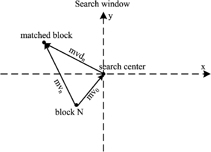
1.

Introduction

Motion estimation (ME) is used in many video coding standards, such as MPEG-1, MPEG-4, and H.264/AVC, to remove interframe redundancies. There are two main factors that determine the performance of ME. One is the size of the search range (SR), and the other is the number of reference frames (RFs). The values of these two factors are set manually in the configuration file of the encoder and are used as fixed parameters in the whole ME process. Although larger SR and RF values enable better coding performance, they also impose a heavy encoding complexity. In the overall coding system, about 50% of the computation time and 90% of the memory access are dedicated to ME.^1,2 Indeed, the memory access bandwidth required to read reference pixels from external memory has gradually become the bottleneck of real-time applications.

Because the coding video differs considerably, fixed SR and RF settings are not suitable for all situations. For example, if the video sequence is motionless, a small SR and single RF are sufficient to determine the best motion vector (MV). On the other hand, if the sequence contains a high degree of movement, we can adaptively adjust the above settings to achieve better video quality. In such cases, dynamic SR adjustment and multiframe selection algorithms have become important in improving coding efficiency and satisfying the needs of real-time applications.

Many algorithms that adaptively adjust the SR size and select the RFs have been proposed. For instance, the influence of the SR on the compression rate and coding quality has been examined in an extensive series of experiments.³ The maximum-likelihood estimator has been used to model the probability density function of the motion vector difference (MVD), with the optimal SR then calculated for a given hitting probability.^4,5 However, the integral operation and likelihood estimator make the algorithm somewhat complicated. In Ref. 6, images are divided into motionless and moving regions, and different SR selection methods are given for each. Using the spatial correlation, the SR can be set as a function of the maximum of the neighboring matching errors.⁷ Similarly, the block can be classified as motionless, slow, or violent based on the magnitude of the predicted motion vector (PMV), allowing a $3\times 3$, $7\times 7$, or $9\times 9$ search area to be selected accordingly.^8,9 In Ref. 10, three different SRs are selected based on certain thresholds. However, with only a few fixed SRs and thresholds, the adaptability of these algorithms^8–10 is insufficient to cope with the diversity of video sequences. In Ref. 11, the correlation between different block partitions is used to predict the SR size. The SR of the current block has been calculated based on the relationship between the probability density function of MVD and the MV distribution of the neighboring blocks.¹² An analysis of the relationship between the compression ratio and the size of the SR has been shown to allow a smaller SR for macroblocks (MBs) with smaller compression ratios.¹³ In Ref. 14, a linear SR model is defined based on the 1-bit image plane.

Existing multiframe selection algorithms are generally classified into three categories. In the first, the MV composition technique is used to reduce the calculation load of multiframe ME, which uses the MVs from the previous RFs to generate those for the current RF. The activity dominant vector selection criterion can be used to obtain the composited MV.¹⁵ The MVs of two successive frames can synthesize the MV of the current RF,¹⁶ with only a small range around the composited MV needed for ME. In Ref. 17, the MVs with the same characteristics are first merged and then the two most relevant MVs are selected to generate the MV of the current block. To apply the MV composition algorithm, the MVs of different block types must be stored for further calculation. Therefore, this approach inevitably involves a large additional memory space.

In the second category, the candidate reference frames (CRFs) are predicted from the temporal and spatial neighbors. The priorities of all RFs can be computed from the spatial and temporal correlation of the RF index and MVs,¹⁸ or the coding modes and RFs from some reference region may be used to determine the CRFs for the current block.¹⁹ In Ref. 20, the initial RF is dynamically selected using the mean of the RF indexes of spatially neighboring MBs.

The third category speeds up the multiframe selection procedure by employing an early termination strategy. For instance, based on the spatial and temporal consistencies of the motion field, multiframe ME may only be selected for a small region of the MBs,²¹ or the experimentally obtained sum of absolute difference (SAD) curve could be used to skip the third and fourth RFs.²² In Ref. 23, the relationship between the SAD and the all-zero quantized transform coefficients was deduced. If the SAD is less than some threshold, the multiframe ME procedure should be terminated immediately. Alternatively, the MVs and SADs from previous RFs can be used to automatically confirm whether to search the last two RFs.²⁴

Different from the above-mentioned methods, we propose a different dynamic SR and multiframe selection algorithm for the H.264/AVC ME process. For the SR adjustment scheme, we first analyze the relationship between the PMV and the SR and then use this relationship to adjust the SR size. For the multiframe selection scheme, we focus on the correlation between different block sizes of the MB to adaptively select RFs. Simulation results show that the proposed algorithm achieves a higher speedup while maintaining almost the same video quality and total bit rate.

The rest of this paper is organized as follows. Sections 2 and 3 describe the algorithms for dynamic SR adjustment and multiframe selection, respectively. Our simulation results are presented in Sec. 4, and we give our conclusions in Sec. 5.

2.

Proposed SR Adjustment Algorithm

2.1.

Motivation and Analysis

The SR size can be successfully reduced using the algorithms mentioned in Sec. 1, but the efficiency can be further improved. In the H.264/AVC coding standard, the PMV decides the center of a search area. Therefore, the SR size depends on the location of the PMV more than any other factors, such as the maximum matching error⁷ or the motion activity.⁸ The relationship between the SR and the PMV is illustrated in Fig. 1. The vector ${\mathrm{mv}}_0$ denotes the search center and is calculated as the median operator over the neighboring MVs, and ${\mathrm{mv}}_n$ is the final MV of block $N$ obtained by ME. The vector $\mathrm{mv}{d}_n$ is the difference between ${\mathrm{mv}}_0$ and ${\mathrm{mv}}_n$. Intuitively, when PMV (${\mathrm{mv}}_0$) is accurate (i.e., when ${\mathrm{mv}}_0$ is close to ${\mathrm{mv}}_n$), fewer regions need to be searched before the final motion vector (${\mathrm{mv}}_n$) is obtained. Hence, we can consider an adaptive SR adjustment algorithm which depends on the PMV.

Fig. 1

Relationship between the search range (SR) and PMV.

To determine an MV within the search window, SAD has been widely used to measure the prediction distortion between the current and the candidate blocks. For a block of size $W\times H$ SAD is defined as

Eq. (1)

$$\mathrm{SAD}[c,r(\mathrm{mv})]=\sum _{i=m,j=n}^{m+W,n+H}|\mathrm{curr}(i,j)-\mathrm{ref}(i+\mathrm{mv}x,j+\mathrm{mv}y)|$$

where $\mathrm{curr}(i,j)$ denotes the pixel value of the current block and ref ($i+\mathrm{mv}x$, $j+\mathrm{mv}y$) is the pixel value of the candidate block for a given motion vector $\mathrm{mv}(\mathrm{mv}x,\mathrm{mv}y)$. In our scheme, we define the Dif metric to evaluate the accuracy of the PMV. In other words, we use Dif to measure the distance between the MV and its predictor. It is defined as follows:

Eq. (2)

$$\mathrm{Dif}=|{\mathrm{SAD}}_I[c,r({\mathrm{mv}}_0)]-{\mathrm{SAD}}_I[c,r({\mathrm{mv}}_i)]|,$$

where ${\mathrm{SAD}}_I[c,r({\mathrm{mv}}_0)]$ and ${\mathrm{SAD}}_I[c,r({\mathrm{mv}}_i)]$ are the SADs computed at the PMV (${\mathrm{mv}}_0$) and the MV (${\mathrm{mv}}_i$) of block $I$, respectively. A small Dif value implies an accurate predictor. Thus, we may expect a high probability of a small SR. To reveal the relationship between Dif and the SR size, the experimental results from a variety of video sequences are shown in Fig. 2. In this figure, $|\mathrm{mv}{d}_n|$ represents the magnitude of the difference between MV and PMV, and $\mathrm{average}\_\mathrm{Dif}$ is the average Dif value of blocks with the same $|\mathrm{mv}{d}_n|$. A clear positive correlation can be seen, especially for $|\mathrm{mv}{d}_n|$ values up to 11. Although $\mathrm{average}\_\mathrm{Dif}$ does not increase monotonously over the whole $|\mathrm{mv}{d}_n|$ range, there is a high probability that $\mathrm{average}\_\mathrm{Dif}$ will become larger as $|\mathrm{mv}{d}_n|$ increases. Hence, we can develop an adaptive SR selection algorithm, which uses Dif as the criterion for determining the SR. That is, the small Dif means the accurate PMV and the small SR value, whereas the large Dif means the large SR value.

Fig. 2

Relationship between Dif and $|{\mathrm{mv}d}_n|$. (Test conditions: encoded $\text{frame}=100$; number of reference $\text{frames}(\mathrm{RFs})=1$; quantization parameter $(\mathrm{QP})=28$; $\mathrm{SR}=16$; group structure is IPP.)

For the current block $N$ in Fig. 1, ${\mathrm{mv}}_n$ is not available until the ME process has been performed across the whole search area, so we must set a predictor for ${\mathrm{SAD}}_N[c,r({\mathrm{mv}}_n)]$ before it can be used. The influence of this predictor on coding quality and efficiency is briefly analyzed as follows. In Eq. (2), if a larger predictor is selected for ${\mathrm{SAD}}_N[c,r({\mathrm{mv}}_a)]$, a smaller Dif value will be obtained. According to Fig. 2, this should result in a smaller SR size. Although a higher coding speed can be achieved with a smaller SR, the coding quality may be lost if the true MV falls outside this smaller SR. In contrast, a smaller predictor gives a larger SR and a higher coding quality. Hence, our purpose is not to get an accurate estimate for ${\mathrm{SAD}}_N[c,r({\mathrm{mv}}_n)]$ but to achieve a tradeoff between the coding quality and the coding efficiency. Therefore, we replace ${\mathrm{SAD}}_N[c,r({\mathrm{mv}}_n)]$ with a smaller predictor:

Eq. (3)

$$\begin{gathered} {\mathrm{SAD}}_N[c,r({\mathrm{mv}}_n)]=\min \{[{\mathrm{SAD}}_A[c,r({\mathrm{mv}}_a)],{\mathrm{SAD}}_B[c,r({\mathrm{mv}}_b)], \\ {\mathrm{SAD}}_C[c,r({\mathrm{mv}}_c)],{\mathrm{SAD}}_E[c,r({\mathrm{mv}}_e)]\} \end{gathered}$$

where ${\mathrm{SAD}}_A[c,r({\mathrm{mv}}_a)]$, ${\mathrm{SAD}}_B[c,r({\mathrm{mv}}_b)]$, ${\mathrm{SAD}}_C[c,r({\mathrm{mv}}_c)]$, and ${\mathrm{SAD}}_E[c,r({\mathrm{mv}}_e)]$ are the SADs computed from the MVs of the spatially neighboring blocks (A is the left block, B is the upper block, C is the upper-right block) and the colocated block (E).

To estimate the SR size of block $N$, let ${\mathrm{Dif}}_N$, ${\mathrm{Dif}}_A$, ${\mathrm{Dif}}_B$, ${\mathrm{Dif}}_C$, and ${\mathrm{Dif}}_E$ denote the Dif values of the current block $N$ and its four neighbors (left, upper, upper-right, and colocated block), respectively. ${\mathrm{Dif}}_A$, ${\mathrm{Dif}}_B$, ${\mathrm{Dif}}_C$, and ${\mathrm{Dif}}_E$ are subtracted from ${\mathrm{Dif}}_B$, ${\mathrm{Dif}}_C$, and ${\mathrm{Dif}}_N$, and the four differences are collected in the set $\mathrm{\Delta }\mathrm{Dif}$:

Eq. (4)

$$\mathrm{\Delta }\mathrm{Dif}=\{{\mathrm{Dif}}_N-{\mathrm{Dif}}_i\},i=A,B,C,\mathrm{and}E\mathrm{.}$$

The SR is then adjusted according to the following conditions.

Condition 1: If any element in $\mathrm{\Delta }\mathrm{Dif}$ is smaller than 0, ${\mathrm{Dif}}_N$ is smaller than the Dif value of (at least) one of its four neighbors. Thus, it can be determined that the PMV of block $N$ is closer to its MV than its neighbor, and therefore the following smaller SR should be set for block $N$:

Eq. (5)

$$\mathrm{SR}=\max [1,\min ({\mathrm{SR}}_A,{\mathrm{SR}}_B,{\mathrm{SR}}_C,{\mathrm{SR}}_E)]\mathrm{.}$$

In Eq. (5), ${\mathrm{SR}}_A$, ${\mathrm{SR}}_B$, ${\mathrm{SR}}_C$, and ${\mathrm{SR}}_E$ are the SRs of blocks A, B, C, and E, respectively.

Condition 2: If all elements in $\mathrm{\Delta }\mathrm{Dif}$ are greater than 0 and ${\mathrm{Dif}}_N>\alpha \times \max ({\mathrm{Dif}}_A,{\mathrm{Dif}}_B,{\mathrm{Dif}}_C,{\mathrm{Dif}}_E)$, where $\alpha$ is an adjustment parameter, the PMV of the current block $N$ is far from its MV, which is likely to be due to complex motion. In such cases, in order to guarantee the coding quality, a larger SR should be set as follows:

Eq. (6)

$$\mathrm{SR}=\min [R,\max ({\mathrm{SR}}_A,{\mathrm{SR}}_B,{\mathrm{SR}}_C,{\mathrm{SR}}_E)+\frac{R}{8}],$$

where $R$ is a fixed SR given in the configuration file of the encoder. Based on extensive experiments, we set the value of $\alpha$ to 2.

Condition 3: If conditions 1 and 2 are not satisfied, the two minimum elements in $\mathrm{\Delta }\mathrm{Dif}$ (corresponding to the blocks that have the closest Dif values to the current block $N$) are selected. These blocks are marked $b_1$ and $b_2$, and the SR of block $N$ is set according to

Eq. (7)

$$\mathrm{SR}=\min [R,\max ({\mathrm{SR}}_{b1},{\mathrm{SR}}_{b2})+1],b1,b2\in \{A,B,C,E\}$$

After determining the new SR according to Eqs. (5)–(7), the ME is performed within this new SR.

3.

Proposed Multiframe Selection Algorithm

3.1.

Motivation and Analysis

Figure 3 describes the relationship between multiframe and variable block size ME. As shown in Fig. 3, the multiframe ME process is performed on each block size of the MB. These blocks are different partitions of the same MB, so their best RFs are highly correlated. According to this feature, the best RFs of the upper divisions can be used as CRFs for the lower divisions. However, using this up-to-down method to predict the CRFs of the lower divisions has two shortcomings. First, if the MB contains the object boundary or the complex content, then the probability that the lower and upper divisions will share the same best RF will be small. Second, the lower partitions have more sub-blocks than the upper partitions. Therefore, this up-to-down prediction method is not very efficient. For example, the $\mathrm{P}8\times 8$ division contains 36 sub-blocks in total. If the number of CRFs is 2, then the 36 sub-blocks will require 72 ME procedures, whereas for the $16\times 16$ division, only two ME procedures are required. Therefore, reducing the number of CRFs in the lower divisions is critical for improving the efficiency of ME.

Fig. 3

Multiple RFs motion estimation (ME) with various block size.

In summary, the $8\times 8$ block is used as the basic unit in this study to determine the best RFs for the other coding modes. We use the $8\times 8$ block as it better reflects the motion and texture characteristics of the MB and improves the efficiency as much as possible. For convenience, the RFs are hereafter marked as ${\mathrm{ref}}_0{,\mathrm{ref}}_1{,\mathrm{ref}}_2{,\mathrm{ref}}_3\dots$ in accordance with their distance from the current frame.

Due to the temporal consistency of a video sequence, it is highly probable that blocks in static or slow-moving regions will select ref₀ as the optimal RF. In this work, the movement complexity (MC) of the MB is defined as

Eq. (8)

$$\mathrm{MC}=\max (|{\mathrm{MV}}_0|,|{\mathrm{MV}}_1|,|{\mathrm{MV}}_2|,|{\mathrm{MV}}_3|),$$

where ${\mathrm{MV}}_0$, ${\mathrm{MV}}_1$, ${\mathrm{MV}}_2$, and ${\mathrm{MV}}_3$ denote the MVs of four $8\times 8$ blocks at ${\mathrm{ref}}_0$.

To inspect the relationship between movement complexity and ${\mathrm{ref}}_0$, various video sequences with different motion activities are used as the test material. Table 2 documents the average experimental results for different QPs. $\mathrm{T}\_\mathrm{B}$ is the number of blocks with the same movement complexity, and RF_ratio represents the percentage of blocks whose ultimate RF is ${\mathrm{ref}}_0$. For the static blocks (which MC is equal to 0), an average of 97.87% of them select ${\mathrm{ref}}_0$ as the best RF. For the News, Container, and Akiyo sequences, the percentage of blocks choosing ${\mathrm{ref}}_0$ among $\mathrm{T}\_\mathrm{B}$ is greater than 99%. Table 2 also shows that the $\mathrm{RF}\_\mathrm{ratio}$ decreases as the value of MC increases. For the Stefan sequence, in particular, when the MC is 3, only 68.32% of $\mathrm{T}\_\mathrm{B}$ select ${\mathrm{ref}}_0$ as their ultimate RF. Therefore, we can conclude that when the value of MC is less than some threshold Th (set to 2 in this paper), there is a very high probability that only ${\mathrm{ref}}_0$ will be used as the best RF. From this result, we conclude that the search across other RFs can be skipped.

Table 2

Relationship between the movement complexity and ref0 (test conditions: encoded frame=60; number of RFs=5; QP=28, 32, 36, 40; SR=16; group structure is IPP).

Sequence	$\mathrm{MC}=0$	$\mathrm{MC}=1$	$\mathrm{MC}=2$	$\mathrm{MC}=3$
	$\mathrm{T}\_\mathrm{B}/\mathrm{RF}\_\text{ratio}$ (%)	$\mathrm{T}\_\mathrm{B}/\mathrm{RF}\_\text{ratio}$ (%)	$\mathrm{T}\_\mathrm{B}/\mathrm{RF}\_\text{ratio}$ (%)	$\mathrm{T}\_\mathrm{B}/\mathrm{RF}\_\text{ratio}$ (%)
$\mathrm{Akiyo}\_\mathrm{Cif}$	$\mathrm{264,189}/99.58$	$\mathrm{86,128}/97.30$	$\mathrm{29,605}/91.85$	$\mathrm{25,107}/91.52$
$\mathrm{Foreman}\_\mathrm{Cif}$	$\mathrm{43,255}/95.07$	$\mathrm{19,532}/90.63$	$\mathrm{18,055}/86.83$	$\mathrm{25,834}/84.51$
$\mathrm{News}\_\mathrm{Cif}$	$\mathrm{225,201}/99.41$	$\mathrm{98,559}/96.78$	$\mathrm{29,105}/91.80$	$\mathrm{24,615}/92.47$
$\mathrm{Container}\_\mathrm{Cif}$	$\mathrm{235,774}/99.01$	$\mathrm{118,000}/93.43$	$\mathrm{45,186}/84.95$	$\mathrm{19,903}/87.60$
$\mathrm{Stefan}\_\mathrm{Cif}$	$\mathrm{49,608}/95.92$	$\mathrm{39,998}/86.18$	$\mathrm{27,724}/73.45$	$\mathrm{29,338}/68.32$
$\mathrm{Highway}\_\mathrm{Cif}$	$\mathrm{213,324}/96.31$	$\mathrm{34,260}/90.09$	$\mathrm{12,538}/85.63$	$\mathrm{25,929}/84.60$
$\mathrm{Flower}\_\mathrm{Cif}$	$\mathrm{128,911}/98.90$	$\mathrm{3,350}/91.39$	$\mathrm{2,658}/90.26$	$\mathrm{14,392}/87.08$
$\mathrm{Silent}\_\mathrm{Cif}$	$\mathrm{170,445}/99.00$	$\mathrm{114,479}/97.77$	$\mathrm{34,214}/93.76$	$\mathrm{26,529}/90.71$
$\mathrm{Hall}\_\mathrm{Cif}$	$\mathrm{242,229}/99.61$	$\mathrm{112,543}/92.41$	$\mathrm{20,033}/89.84$	$\mathrm{12,179}/86.87$
Average	$/97.87$	$/92.87$	$/87.60$	$/86.00$

If MC is larger than Th, it indicates that the motion is complex. Thus, we perform ME on the remaining RFs for each $8\times 8$ block. The reference maps are then generated according to the correlation between the $8\times 8$ block and the other blocks. Figure 4 shows the reference maps for other blocks, where ${\mathrm{ref}}_a$, ${\mathrm{ref}}_b$, ${\mathrm{ref}}_c$, and ${\mathrm{ref}}_d$ denote the optimal RFs of the first, second, third, and fourth $8\times 8$ block, respectively. The CRFs for each partition are described as follows:

• a. The $\mathrm{P}16\times 16$ mode is used to encode regions containing slow motion. Thus, if more than two RFs are contained in Fig. 4(a), the motion of the current block is complex and the $\mathrm{P}16\times 16$ mode cannot be selected. In this case, only ${\mathrm{ref}}_0$ is selected as the best RF; otherwise all RFs contained in Fig. 4(a) are selected as CRFs for the $16\times 16$ block.

• b. For the $16\times 8$ block, ${\mathrm{ref}}_a$ and ${\mathrm{ref}}_b$ are regarded as CRFs for the upper $16\times 8$ division, whereas ${\mathrm{ref}}_c$ and ${\mathrm{ref}}_d$ are CRFs for the lower $16\times 8$ division in Fig. 4(b).

• c. For the $8\times 16$ block, ${\mathrm{ref}}_a$ and ${\mathrm{ref}}_c$ are regarded as CRFs for the left $16\times 8$ division, whereas ${\mathrm{ref}}_b$ and ${\mathrm{ref}}_d$ are CRFs for the right $16\times 8$ division in Fig. 4(c).

• d. For the three $8\times 8$ subdivisions, the best RF for the $8\times 8$ block is directly used as the best RF for its subdivisions in Fig. 4(d).

Fig. 4

Reference maps of different partitions.

3.2.

Proposed Algorithm

Based on the above description, the pseudocode for our multiframe selection algorithm can be written as shown in Fig. 5. The initial number of CRFs is usually set to 5.

Fig. 5

Pseudocode for our algorithm.

As shown in Fig. 5, ME is first performed on ${\mathrm{ref}}_0$ for the four $8\times 8$ blocks, and the MVs of the four blocks are used to calculate the motion complexity according to Eq. (8). If MC is less than the threshold Th (set as 2), then ${\mathrm{ref}}_0$ is set as the CRF. Otherwise, ME is conducted on from ${\mathrm{ref}}_1$ to ${\mathrm{ref}}_4$ for the four $8\times 8$ blocks, respectively. The next step is to determine a candidate reference frames set (CRFS) for other partitions based on the reference maps in Fig. 4. ME is then performed on the RFs in the CRFS for the $8\times 8$ sub-block, $16\times 16$ block, $16\times 8$ block, and the $8\times 16$ block. In the ME process for H.264/AVC, the coding order is $\mathrm{P}16\times 16$, $\mathrm{P}16\times 8$, $\mathrm{P}8\times 16$, and then $\mathrm{P}8\times 8$. As the proposed algorithm changes the coding order, i.e., the $8\times 8$ block is processed first, the MVs of the second, third, and fourth $8\times 8$ blocks must be repredicted after finishing the whole ME process, otherwise there will be some inconsistency between the decoder and encoder.

Using the pseudocode above, we investigate the number of RFs under the best- and worst-case scenarios. In the best case, only one RF (${\mathrm{ref}}_0$) is required for all block divisions. In the worst case, all five RFs are required for the $8\times 8$ blocks; each of the $16\times 16$ block, $16\times 8$ block, and $8\times 16$ block have two CRFs. However, subpartitions such as $8\times 4$, $4\times 8$, and $4\times 4$ will always have one RF. Therefore, the average number of RFs required for the entire coding of the MB is $[(4\times 5)+(1\times 2)+(2\times 2)+(2\times 2)+(16\times 1)+(8\times 1)+(8\times 1)]/41\approx 1.51$.

To verify the effectiveness of the above method, the average hit ratio for different QPs at each block size was compared to the full RF search method. The results are shown in Table 3. As can be seen, our algorithm achieves a high average accuracy of 91% to 98% for all block partitions. For the $16\times 16$ block size, the hit ratio averages above 95%. Even the $8\times 8$ sub-block averages over 91%, with a worst-case performance of 84.75% with the Mobile sequence.

Table 3

Average hit ratios of the proposed algorithm for each block size (test conditions are the same as Table 2).

Sequence	$\mathrm{P}16\times 16$	$\mathrm{P}16\times 8$	$\mathrm{P}8\times 16$	$\mathrm{P}8\times 8$	Sub-$\mathrm{P}8\times 8$
$\mathrm{Akiyo}\_\mathrm{Cif}$	98.31	97.91	97.82	99.58	96.60
$\mathrm{News}\_\mathrm{Cif}$	98.23	97.43	97.22	99.12	95.76
$\mathrm{Stefan}\_\mathrm{Cif}$	92.17	91.21	90.76	97.68	88.06
$\mathrm{Forman}\_\mathrm{Cif}$	92.17	90.00	89.37	97.94	87.32
$\mathrm{Hall}\_\mathrm{Cif}$	97.35	97.20	96.96	98.63	96.34
$\mathrm{Mobile}\_\mathrm{Cif}$	95.52	90.65	89.48	98.07	84.75
$\mathrm{Container}\_\mathrm{Cif}$	97.21	96.67	96.79	99.09	95.35
$\mathrm{Paris}\_\mathrm{Cif}$	97.24	95.76	95.87	98.92	93.16
$\mathrm{Coastguard}\_\mathrm{Cif}$	96.18	92.37	93.14	99.08	90.13
Average	95.76	93.91	93.70	98.57	91.36

4.

Simulation Results and Analysis

To evaluate the performance of the proposed approach, it was implemented on the H.264/AVC reference software JM15.1. Various standard sequences were used, including CIF, 4CIF, and HD sizes, at 30 fps for 100 frames. The simulations were performed with rate distortion (RD) optimization and Hadamard transform enabled, $\mathrm{QP}=28$, 32, 36, and 40, IPPP sequence types, CAVLC entropy coding, and one or five RFs. The default SR was set to 16 for CIF, 32 for 4CIF, and 64 for HD sequences.

For a numerical comparison, the Bjontegaard delta peak signal-to-noise ratio (BDPSNR) and Bjontegaard delta bit rate (BDBR) were used to evaluate the coding quality. These quantities are recommended for comparing the difference between two RD curves.²⁵ A negative BDPSNR (dB) or positive BDBR (%) indicates a coding loss over the full-search algorithm in JM15.1. For an objective comparison, the average used reference frame (URF) and average computational complexity (CPX) are used to measure the complexity reduction. CPX (%)⁴ is the speed-up ratio of the SR adjustment algorithm, which is defined as the ratio of the number of search points in the proposed method to the number of search points in the full-search motion estimation (FME) algorithm. For example, a CPX value of 21% implies that the number of search points in the proposed method is 21% of the number in the FME algorithm. The average URF represents the average number of RFs used by each MB, with a smaller URF signifying fewer RFs.

For an objective comparison of coding performance, the proposed approach was compared with corresponding methods. Our SR adjustment method was compared to two recent schemes.^4,11 It can be seen from Table 4 that the proposed algorithm reduced the number of search points by an average of 2.56%, albeit at the cost of a 0.14% increase in bit rate and a 0.06 dB reduction in peak signal-to-noise ratio (PSNR). When the hitting probability of MVDs was set to 0.7, the method of Ko et al.⁴ exhibited a good performance, with an average CPX of 4.94%. However, the implementation cost of this method is much higher than that of the proposed scheme due to the overheads inherent in the integral operation and likelihood estimation. For several sequences, such as Stefan, $\mathrm{Station}2\_\mathrm{Hd}$, and $\mathrm{Soccer}\_4\mathrm{Cif}$, the method of Ref. 11 exhibited better coding quality than our method in terms of BDPSNR and BDBR, but our approach can further deduct an average of 11% search points with only a slight bit rate increase and small PSNR decrease.

Table 4

Performance comparison of the proposed algorithm on JM 15.1 (with one RF).

For further comparison, Table 5 depicts the ME time of the proposed method compared to the UMHexagonS algorithm in JM15.1. This shows that the proposed method reduces the ME time by 9.15% on average, with a marginal increase in BDBR ($+0.07\%$) and a small loss of BDPSNR ($-0.01\mathrm{dB}$). For sequences with static and slow motion activity, such as $\mathrm{Akiyo}\_\mathrm{Cif}$ and $\mathrm{Hall}\_\mathrm{Cif}$, UMHexagonS achieves a high speed-up factor, because the ME process is terminated after finishing the small and middle diamond pattern search. In contrast, our algorithm works well for CIF sequences with high motion levels and 4CIF and HD sequences with larger SR values.

Table 5

Performance comparison with UMHexagonS algorithm (test conditions are the same as Table 4).

We compared our multiframe selection algorithm with two well-known efficient algorithms.^19,23 The comparison results are listed in Table 6. For most sequences, the method of Lee et al.¹⁹ yielded a high bit rate increment and PSNR loss (average of 0.09 dB BDPSNR decrease and 0.61% BDBR increase), with 1.88 frames searched compared to the JM15.1 reference encoding. The method of Ref. 23 achieved good PSNR and bit rate performance (average 0.06 dB BDPSNR decrease and 0.45% BDBR increase) with a higher speed-up factor (1.52 RFs used). The proposed algorithm gave superior results to both of these techniques in terms of coding complexity reduction. It outperformed the method of Lee et al.¹⁹ in all aspects, with a 0.63-frame reduction in the number of searched RFs, which implies a reduction of 12% in the number of ME operations. At the same time, the proposed method improved the URF value by 0.31 frames compared to the method of Huang et al.,²³ with a better bit rate and the same PSNR.

Table 6

Performance comparison of the proposed algorithm on JM 15.1 (with five RFs).

It should be mentioned that the URF and CPX parameters are virtually independent of the programming quality or hardware platform. Therefore, it is clear that the performance of the proposed methods is superior to the corresponding methods evaluated above. It must also be noted that the proposed methods can be combined with any fast ME method, such as Fast Full search, EPZS, and UMHexagonS, in the JM reference encoder.

5.

Conclusions

In this paper, we presented an efficient adaptive SR adjustment and multiframe selection algorithm for ME. The proposed SR adjustment algorithm adjusts the SR for ME based on the accuracy of PMV. We also designed an RF selection scheme with the aim of reducing the complexity of multiframe ME based on the relationship between the different block sizes of the MB. The described technique significantly reduces the CPX of ME in H.264/AVC. Through a comparative analysis, it was found that the proposed approach gave an average RF saving of 3.75 frames (1.25 URFs) with a setting of five RFs and a reduction of 97% in the number of search points with a setting of one RF, with a negligible bit rate increment and a minimal loss of image quality. These features will be important in the development of real-time coding applications for video conferencing and telephony. In future work, we will combine our two algorithms to further speed up the ME process.