1.

Introduction

Breast magnetic resonance imaging (MRI) has gradually gained much popularity in clinical use because results have shown that the screening accuracy of MRI is significantly higher than that of mammography and ultrasound.¹ Currently, doctors generally rely on breast MRI for obtaining the region of tumor since it is usually an important sign of breast cancer for diagnosis. Based on these considerations, this study proposes a new scheme that adopts mathematical algorithms from multispectral image processing techniques for specific object contrast enhancement. The tumor region can be segmented from contrast-enhanced images and shown as a binary image. We anticipate that the generated binary tumor region images will aid doctors in clinical diagnosis.

Over the years, many computer-assisted methods have been developed for analyzing single-spectral MRI, such as principal component analysis (PCA),² eigenimage analysis,³ neural networks,⁴ and fuzzy c-means (FCMs).⁵ Eigenimage analysis has been shown to be effective in segmentation and feature extraction, and neural networks have been found to perform well in segmenting brain tissues and have been compared with classical maximum likelihood methods. However, because multispectral images provide more information for processing or analysis, multispectral analysis techniques can be used to improve the performance. Hence, several methods have been developed for processing multispectral MRIs, such as orthogonal subspace projection (OSP)⁶ and Kalman filter,⁷ but both of them require prior knowledge. With these considerations, we have developed a new method called the independent component texture analysis (ICTA) to segment the tumor region in multispectral breast MRIs. ICTA comprises three techniques: independent component analysis (ICA), entropy-based thresholding (ET), and texture feature registration (TFR). Among them, ICA, originally, is a blind source separation (BSS) method in the signal processing field, and it is a powerful tool for feature extraction and data representation such as speech recognition, image recognition, and statistical analysis.⁸

The proposed method initially assumes multispectral breast MRIs to be gray-level values in a three-dimensional space composed of several independent components (ICs) that can be regarded as different tissues of the breast such as fat, glands, tumor mass, and muscle. First, the ICA technique is used to separate the ICs. Second, the binary images that indicate the suspicious tumor region are generated using the ET technique. Finally, texture feature extraction is employed to find the consistency of the tumor texture feature in suspicious tumor regions, which is called TFR. The texture features adopted for feature description are called the texture spectrum (TS), which is based on the varying relationship between the gray levels of both image pixels and surrounding pixels. We divided the TS according to three feature descriptors named black-white symmetry (BWS), geometric symmetry (GS), and degree of direction (DD).⁹ According to the experimental results, the three feature values may effectively reflect differences between tumors and normal tissues. The binary image of the tumor region selected by TFR is the output of proposed ICTA method that could assist doctors in their diagnosis. A flowchart of the proposed ICTA is shown in Fig. 1. The performance of ICTA is compared with that of principal component texture analysis (PCTA), FCM, constrained energy minimization (CEM), and OSP methods using a set of breast MRIs to evaluate the feasibility of this new method in medical and clinical applications.

Fig. 1

Flow chart of independent component texture analysis (ICTA).

The remainder of this paper is organized as follows: Sec. 2 presents the existing multispectral image blind separation technique, ICA. Section 3 describes in detail the proposed method, ICTA. Section 4 explains the experiments and their results. Finally, the conclusions are presented in Sec. 5.

2.

Independent Component Analysis

ICA has been developed to solve BSS problems such as the cocktail party problem, and it is an extension of the covariance-based PCA method. The observed signals are considered to be a linear combination of the original signals and a mixing matrix. The goal is to find the mixing matrix. In this paper, we applied the ICA technique to separate multispectral breast MR images of different tissues. First, let us define an $n$-dimensional original signal denoted as a vector $\mathbf{S}={({\mathbf{s}}_{\mathbf{1}},{\mathbf{s}}_{\mathbf{2}},\dots ,{\mathbf{s}}_{\mathbf{n}})}^{\mathbf{T}}$. Through linear transformation, we obtain an $m$-dimensional observed signal denoted as a vector $\mathbf{X}={({\mathbf{x}}_{\mathbf{1}},{\mathbf{x}}_{\mathbf{2}},\dots ,{\mathbf{x}}_{\mathbf{m}})}^{\mathbf{T}}$. We assume that the linear transformation $X$ is composed of a mixing matrix $A$ of size $m\times n$ and the original signal $S$

For simplicity, we rewrite the above equation as follows:

Currently, many algorithms have been developed for the implementation of ICA, but most of them either require complex computation or have slow convergence. In this paper, we applied the fast fixed-point algorithm (FastICA)¹⁰ proposed by Hyvarinen and Oja for the effective implementation of ICA. The principal advantages of this algorithm are fast convergence and simple computation.

3.

Independent Component Texture Analysis

Because ICs generated by ICA are inconsistent and cannot identify tissue automatically, this paper proposes ICTA, which combines ICA, ET, and TFR, to cope with the aforementioned problems of ICA and accordingly determine the target tumor region from ICs. The following sections describe ET and TFR in more detail.

3.1.

Entropy-Based Thresholding

In ICTA, ET (Refs. 11 and 12) is first used to segment suspicious regions from an IC. For a start, we let $t_{ij}$ be the ($i$, $j$)’th element of a co-occurrence matrix $W$ that considers the gray-level transitions between two adjacent pixels. We define it as

Eq. (5)

$$t_{ij}=\sum _{l=1}^M\sum _{k=1}^N\delta (l,k),$$

where

Eq. (6)

$${\delta }_{d,\theta }(l,k)=\{\begin{array}{ll}1,& \text{if}I(l,k)=i,I(l,k+1)=j\text{and}/\text{or}I(l,k)=i,I(l+1,k)=j\\ 0,& \text{otherwise}\end{array}.$$

The probability of a transition from gray level $i$ to $j$ is obtained as

Eq. (7)

$$p_{ij}=\frac{t_{ij}}{\sum _{i=0}^{L-1}\sum _{j=0}^{L-1}{t}_{ij}}.$$

Assume that $t$ is the threshold used to threshold an image. Then, $t$ partitions the co-occurrence matrix defined by Eq. (6) into four quadrants, $A$, $B$, $C$, and $D$, as shown in Fig. 2.

Fig. 2

Co-occurrence matrix with four quadrants divided by threshold $t$.

These four quadrants can be further grouped into two classes. We assume that pixels with gray levels above the threshold are assigned to the foreground (objects) and those equal to or below the threshold are assigned to the background. Quadrants $A$ and $C$ correspond to local transitions within the background and foreground, respectively, whereas quadrants $B$ and $D$ represent transitions across boundaries between the background and foreground. The probabilities associated with each quadrant are then given by

Eq. (8)

$$P_A^t=\sum _{i=0}^t\sum _{j=0}^t{p}_{ij},P_B^t=\sum _{i=0}^t\sum _{j=t+1}^{L-1}{p}_{ij},P_C^t=\sum _{i=t+1}^{L-1}\sum _{j=0}^t{p}_{ij},P_D^t=\sum _{i=t+1}^{L-1}\sum _{j=t+1}^{L-1}{p}_{ij}.$$

The probabilities in each quadrant can be further obtained by so-called cell probabilities:

Eq. (9)

$$p_{ij|A}^t=\frac{p_{ij}}{P_A^t},p_{ij|B}^t=\frac{p_{ij}}{P_B^t},p_{ij|C}^t=\frac{p_{ij}}{P_C^t},p_{ij|D}^t=\frac{p_{ij}}{P_D^t},$$

which are conditional probabilities for a specific quadrant.

Three definitions—local entropy, joint entropy, and global entropy—can be derived on the basis of the cell probabilities, each of which yields a different method. According to experimental results, the threshold obtained from the local entropy is better than that obtained from the joint and global entropies. Therefore, we focused on the local entropy in this study.

3.1.1.

Local entropy

Because quadrants $A$ and $C$ contain local transitions from background to background (BB) and objects to objects (FF), respectively, the local entropy of BB, denoted by $H_{\mathrm{BB}}(t)$, and the local entropy of FF, denoted by $H_{\mathrm{FF}}(t)$, can be defined as

Eq. (10)

$$H_{\mathrm{BB}}(t)=-\sum _{i=0}^t\sum _{j=0}^t{p}_{ij|A}^t\log p_{ij|A}^t,$$

Eq. (11)

$$H_{\mathrm{FF}}(t)=-\sum _{i=t+1}^{L-1}\sum _{j=t+1}^{L-1}{p}_{ij|C}^t\log p_{ij|C}^t.$$

By summing up the local within-class transition entropies of the foreground and the background, a second-order local entropy, denoted by $H_{\mathrm{LE}}(t)$, has been derived by Pal and Pal¹¹ as

Eq. (12)

$$H_{\mathrm{LE}}(t)=H_{\mathrm{BB}}(t)+H_{\mathrm{FF}}(t).$$

The LE method proposed by Pal and Pal¹¹ selects a threshold $t_{\mathrm{LE}}$ by maximizing $H_{\mathrm{LE}}(t)$ as defined in Eq. (12) over $t$ so that

Eq. (13)

$$t_{\mathrm{LE}}=\arg \{\underset{t}{\max }{H}_{\mathrm{LE}}(t)\}.$$

3.2.

Texture Feature Registration

After ICs are segmented by ET, the TS (Ref. 9) is then applied to extract texture features from the segmented region (suspicious region) for identifying the optimum IC. TS is intended for feature description based on the varying relationship between the gray levels of the image pixels and the surrounding pixels. It has shown high efficiency in tissue discrimination. The feature value (TS) calculated from the suspicious region is then compared with the value calculated from a proven tumor region to define its probability and determine the most probable IC, and so is referred to as “TFR.” In TFR, TS is subdivided into three feature descriptors named BWS, GS, and DD,⁹ which are described as follows.

3.2.1.

Texture spectrum

A group of vectors $\mathbf{V}=\{{\mathbf{V}}_{\mathbf{0}},{\mathbf{V}}_{\mathbf{1}},\dots ,{\mathbf{V}}_{\mathbf{8}}\}$ is defined for the pixel of which $V_0$ represents the gray level of the mask central pixel and $V_1,V_2,\dots ,V_8$ represent the gray levels of the surrounding eight points. The relationship $E$ between the central pixel $V_0$ and the surrounding eight pixels is

Eq. (14)

$$E_i=\{\begin{array}{ll}0& \text{if}{V}_i\\ 1& \text{if}{V}_i=V_0\mathrm{for}i=1,2,\dots ,8\\ 2& \text{if}{V}_i>V_0\end{array}.$$

The relationship between the central pixel and its eight adjacent pixels is defined as a texture unit (TU), $\mathrm{TU}=\{E_1,E_2,\dots ,E_8\}$, with each element having three possibilities. Thus, the possible available number of TU is $3^8=6561$, which is associated with a TU code $N_{\mathrm{TU}}$, defined as

Eq. (15)

$$N_{\mathrm{TU}}=\sum _{i=1}^8{E}_i\times 3^{i-1}.$$

The surrounding eight pixels are assigned letters a to h clockwise, as illustrated in Fig. 3. Using the TS, it is possible to define the following texture features that represent the textures of images:

Fig. 3

Assigned letters of texture units for texture spectrum (TS).

BWS:

Eq. (16)

$$\mathrm{BWS}=[1-\frac{\sum _{i=0}^{3279}|S(i)-S(3281+i)|}{\sum _{i=0}^{6560}S(i)}],$$

GS:

Eq. (17)

$$\mathrm{GS}=[1-\frac{1}{4}\sum _{j=1}^4\frac{\sum _{i=0}^{6560}|S_j(i)-S_{j+4}(i)|}{2\times \sum _{i=0}^{6560}{S}_j(i)}],$$

DD:

Eq. (18)

$$\mathrm{DD}=[1-\frac{1}{6}\sum _{m=1}^3\sum _{n=m+1}^4\frac{\sum _{i=0}^{6560}|S_m(i)-S_n(i)|}{2\times \sum _{i=0}^{6560}{S}_m(i)}],$$

where $S(i)$ represents the occurrence frequency of the $i$’th TU code, $i=0,\dots ,6560$ and $S_j(i)$ represents the occurrence frequency of the $i$’th TU code with $j$ as the starting position, $j=1,2,\dots ,8$ (corresponding to $\mathrm{a},\mathrm{b},\dots ,\mathrm{h}$ in Fig. 3).

For the implementation of TFR, the tumor regions of T1, T2, and PD were first identified by experienced radiologists and then the TS was used to extract the texture features from these known tumor regions. Different sections in cases were utilized to obtain the reference tumor texture features. Table 1 shows the texture feature mean values extracted from the proven tumor regions.

Table 1

Mean value of tumor texture features.

Bands	Texture descriptor
	Black-white symmetry	Geometric symmetry	Degree of direction
PD	0.0175	0.6449	0.5649
T1	0.0296	0.6484	0.5203
T2	0.0168	0.7198	0.6026

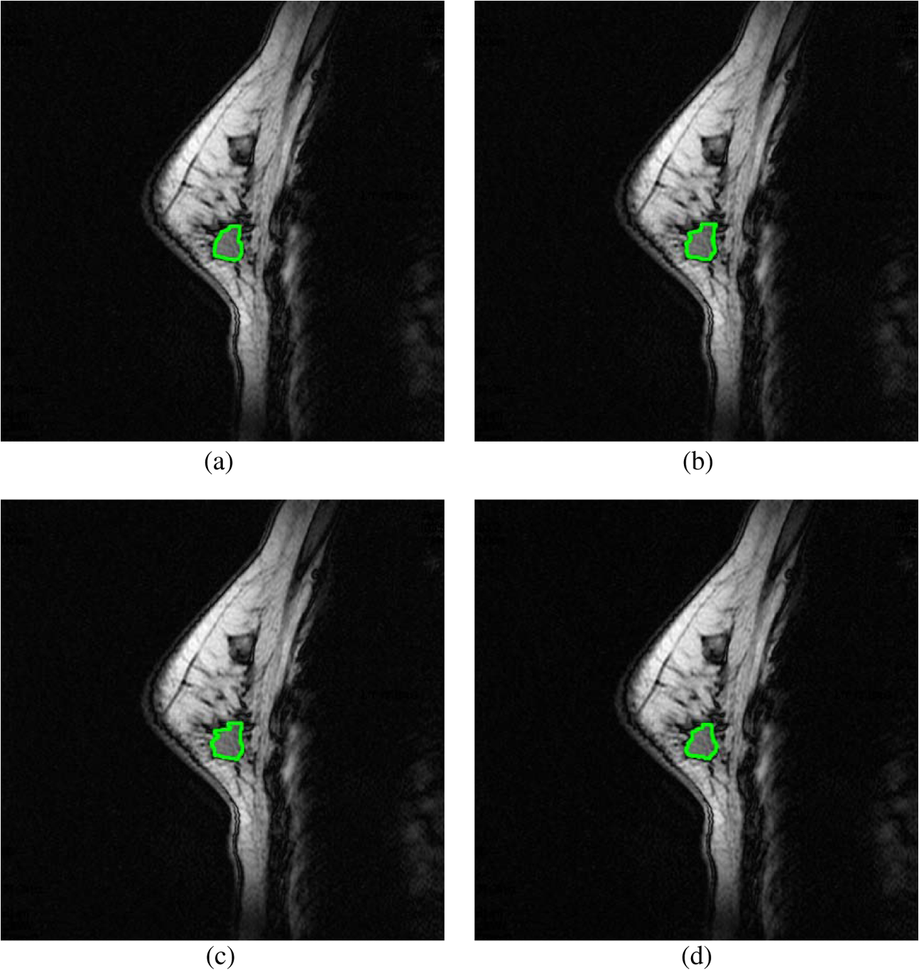
4.

Experimental Results

In this section, the performances of CEM, OSP, FCM, PCTA, and the proposed ICTA are evaluated with breast MRI datasets.

4.1.

Experimental Data

In total, 16 cases of breast MRIs were acquired from Tri-Service General Hospital in Taiwan for performance evaluation, of which 11 cases contain tumor and five cases without tumor. The MRIs were performed on a 1.5T MAGNETOM Vision Plus system (Siemens, Erlangen, Germany). One demonstrated case which contains a medium size tumor is selected as an example and shown in Fig. 4 with four different sequences (bands): PD-weighted spectral image acquired with $\mathrm{TR}/\mathrm{TE}(\text{repetition time}/\text{echo time})=3000/15\mathrm{ms}$, T1-weighted spin-echo image acquired with $\mathrm{TR}/\mathrm{TE}=832/20\mathrm{ms}$, T2-weighted spin-echo image acquired with $\mathrm{TR}/\mathrm{TE}=3000/105\mathrm{ms}$, and T1_FS (T1-weighted fat-saturated image). The resolution and size of each band are 8-bit gray level and $427\times 427$, respectively. The slice thickness of all MRIs is 2 mm.

Fig. 4

A demonstrated case of breast magnetic resonance images (MRIs) which contain a medium-size tumor with four different sequences (bands): PD-weighted (a), T1-weighted (b), T2-weighted (c), and T1_FS (d).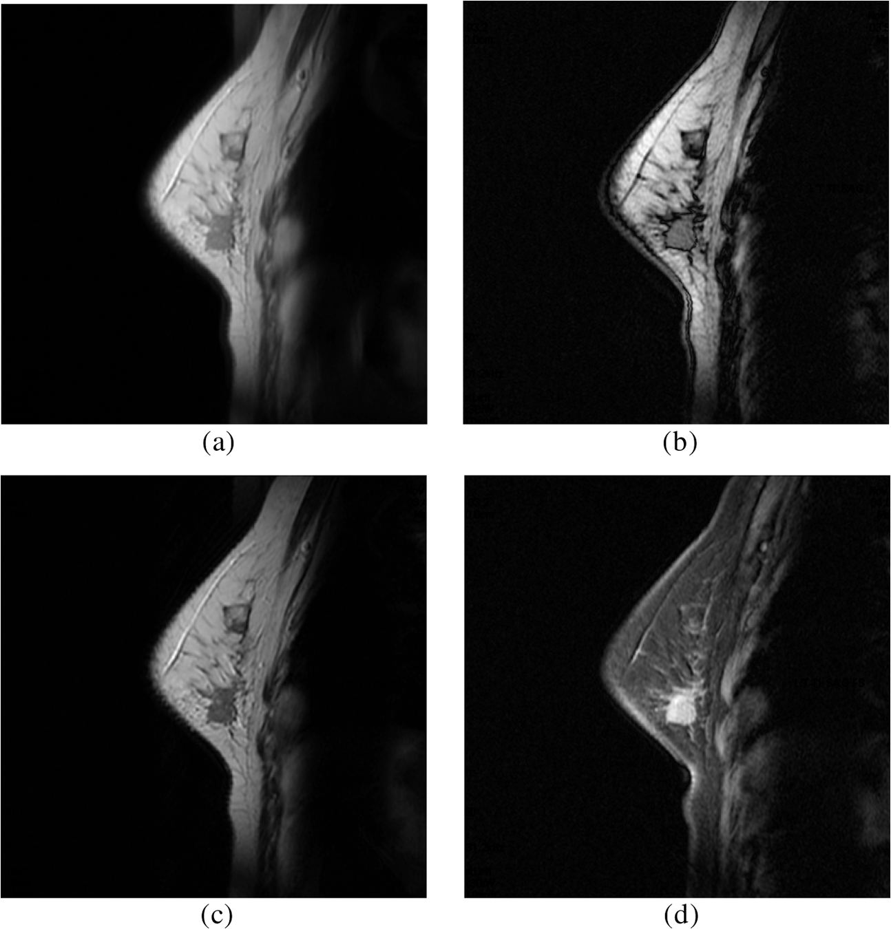

In each case, the standard tumor region required for performance evaluation was conformably verified by three experienced radiologists as shown in Fig. 5(d). In Fig. 5, Fig. 5(a)–5(c) shows the contours of the tumor mass delineated by three experienced radiologists, and Fig. 5(d) is the result of the intersection of Fig. 5(a)–5(c).

Fig. 5

(a)–(c) Contours of tumor mass delineated by three different experienced radiologists. (d) Result of intersection of (a)–(c).

4.3.

Experimental Results

The experimental results obtained by the traditional ICA method are shown in Table 2, where the highest classification rates are given in bold face. In Table 2, four IC and four IC’ (negative film of IC) values are generated in 10 run times. As seen in Table 2, the highest classification rates did not appear in the same IC in each run time. Therefore, the classification rates would not be high as shown in the last row if we chose a fixed IC as the classification result. Table 3 presents the mean values of the 10 highest classification rates manually selected from ICs in 100 run times for three cases with different tumor sizes (big, medium, and small). From the results of Table 3, we can see that the performance of the ICA method was better than the PCA method, but both of them were unable to identify the tumor region by employing a fixed IC.

Table 2

Tumor correct-classification rates of ICA for a case. IC 1’ represents the negative film of IC 1, and so forth.

Run times	IC 1 (%)	IC 2 (%)	IC 3 (%)	IC 4 (%)	IC 1’ (%)	IC 2’ (%)	IC 3’ (%)	IC 4’ (%)
1	31.25	19.28	$\mathbf{99.14}$	25.25	68.75	80.72	0.85	74.76
2	68.76	$\mathbf{99.20}$	27.64	75.20	31.25	0.80	72.33	24.78
3	31.26	$\mathbf{99.20}$	72.34	75.19	68.75	0.80	27.63	24.79
4	31.25	80.72	0.85	74.76	68.76	19.28	$\mathbf{99.14}$	25.25
5	31.25	$\mathbf{99.20}$	27.64	75.19	68.75	0.80	72.33	24.79
6	31.26	80.72	$\mathbf{99.14}$	74.77	68.75	19.28	0.85	25.25
7	68.75	0.80	27.64	75.20	31.25	$\mathbf{99.20}$	72.33	24.79
8	31.26	$\mathbf{99.20}$	72.33	24.78	68.75	0.80	27.64	75.20
9	31.26	$\mathbf{99.20}$	72.34	24.79	68.75	0.80	27.64	75.19
10	68.75	19.28	0.85	25.25	31.26	80.72	$\mathbf{99.14}$	74.76
Average	42.51	$\mathbf{69.68}$	49.99	55.04	57.50	30.32	49.99	44.96

Table 3

Tumor classification rates of ICA and PCA for three demonstrated cases with different tumor sizes (big, medium, and small), by mean values of 10 highest classification rates in 100 run times.

Methods	Case 1 (big) (%)	Case 2 (medium) (%)	Case 3 (small) (%)
ICA	99.17	99.38	91.30
PCA	95.63	99.09	91.03

The texture features calculated from the suspicious tumor region for each IC were then compared with the reference tumor texture features to find out the most probable ICs according to their Euclidean distance calculated as

Eq. (24)

$${\mathrm{IC}}_S^{\mathrm{BWS}}=\sqrt{{({\mathrm{PD}}^{\text{BWS}}-{\mathrm{PD}}_S^{\mathrm{BWS}})}^2+{(T{1}^{\text{BWS}}-T{1}_S^{\mathrm{BWS}})}^2+{(T{2}^{\text{BWS}}-T{2}_S^{\mathrm{BWS}})}^2},$$

Eq. (25)

$${\mathrm{IC}}_S^{\mathrm{GS}}=\sqrt{{({\mathrm{PD}}^{\mathrm{GS}}-{\mathrm{PD}}_S^{\mathrm{GS}})}^2+{(T{1}^{\mathrm{GS}}-T{1}_S^{\mathrm{GS}})}^2+{(T{2}^{\mathrm{GS}}-T{2}_S^{\mathrm{GS}})}^2},$$

Eq. (26)

$${\mathrm{IC}}_S^{\mathrm{DD}}=\sqrt{{({\mathrm{PD}}^{\mathrm{DD}}-{\mathrm{PD}}_S^{\mathrm{DD}})}^2+{(T{1}^{\mathrm{DD}}-T{1}_S^{\mathrm{DD}})}^2+{(T{2}^{\mathrm{DD}}-T{2}_S^{\mathrm{DD}})}^2},$$

where $S$ is the number of ICs, and the texture features distance between ICs and the known tumor is calculated by

Eq. (27)

$${\mathrm{ICTA}}_S=({\mathrm{IC}}_S^{\mathrm{BWS}}+{\mathrm{IC}}_S^{\mathrm{GS}}+{\mathrm{IC}}_S^{\mathrm{DD}})/3$$

with a most probable IC selected using minimum distance as

Eq. (28)

$$\min \{{\mathrm{ICTA}}_1,{\mathrm{ICTA}}_2,\dots ,{\mathrm{ICTA}}_S\}.$$

Table 4 shows the tumor classification rates for all IC and IC’ values of the three cases using traditional ICA, and the minimum distances are given in bold face. From Table 4, we can see that ICs with minimum distance will have highest classification rate. Such a result also indicates that correct ICs could be found by using TFR. Table 5 shows the correct IC identification rates of TFR for 16 cases, of which 11 cases contain tumor and five cases without tumor. According to experimental experience, the result of a case will be identified as no tumor within if all the distances of ICs are $>0.4$.

Table 4

Comparison between classification rate and distance defined in Eq. (27) for three demonstrated cases by using ICA.

Method	Case 1(big)		Case 2 (medium)		Case 3 (small)
	Distance	Tumor classification rates (%)	Distance	Tumor classification rates (%)	Distance	Tumor classification rates (%)
IC 1	0.8423	68.75	0.9527	80.99	0.6094	8.63
IC 2	0.8050	0.80	$\mathbf{0.3462}$	$\mathbf{99.36}$	0.5833	15.99
IC 3	0.8563	27.64	0.4158	60.70	0.8758	73.10
IC 4	0.2553	75.20	0.4548	63.56	0.6181	39.32
IC 1’	0.2552	31.25	1.0990	19.78	$\mathbf{0.3269}$	$\mathbf{91.30}$
IC 2’	$\mathbf{0.1878}$	$\mathbf{99.20}$	1.0999	1.45	0.5185	83.99
IC 3’	0.2077	72.33	1.1421	40.19	0.3983	26.89
IC 4’	0.8388	24.79	1.1330	37.28	0.6962	60.57

Table 5

Correct IC identification rates by using texture feature registration (TFR) calculated in 100 run times for 16 cases (11 contain tumor and five without tumor).

IC identification rates (%)

Correct-classification rate 92.09

False-alarm rate 6.36

Figure 6 shows high-contrast images resulting from ICTA, PCTA, CEM, and OSP methods, where the PCTA method has the same procedure with ICTA, but using PCA instead of ICA. Figure 7 shows ROC curves for the classified sections shown in Fig. 6. Table 6 presents the area under the ROC curves for ICTA, PCTA, CEM, and OSP. Figure 8 shows the segmentation results of applying ICTA, PCTA, CEM, and OSP on the images shown in Fig. 4. In addition, we add an FCM into Fig. 8 for comparison because it is a common representative in classification. Table 7 shows the averaged tumor correct-classification and false-alarm rates obtained from applying ICTA, PCTA, FCM, CEM, and OSP in our experimental data set. From Tables 6 and 7, we can see that ICTA has good performance with lowest false-alarm rate, as does CEM. But unlike CEM, which requires prior knowledge, ICTA is a blind classification technique.

Fig. 6

High-contrast images resulting from the demonstrated case by using ICTA (a), principal component texture analysis (PCTA) (b), constrained energy minimization (CEM) (c), and orthogonal subspace projection (OSP) (d), respectively.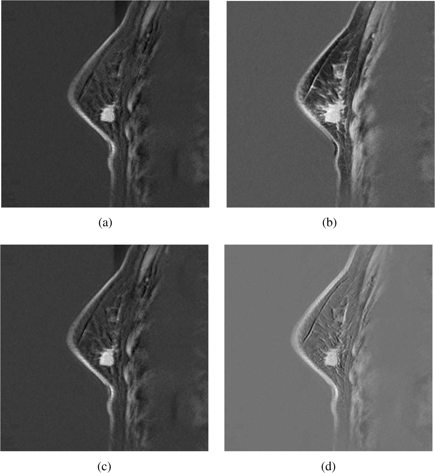

Fig. 7

Receiver operator characteristic (ROC) curves for tumor classification results for the demonstrated case in Fig. 6. (a), Correct-classification rate (RD) versus false-alarm rate (RF). (b), RD versus $\alpha \%$. (c), RF versus $\alpha \%$.

Table 6

Area under ROC curve (RD versus RF) for ICTA, PCTA, CEM, and OSP.

Methods	Case 1 (big)	Case 2 (medium)	Case 3 (small)
Blind source separation
ICTA	0.9920	0.9936	0.9130
PCTA	0.9563	0.9909	0.9103
Prior knowledge required
CEM	0.9935	0.9952	0.9649
OSP	0.9852	0.9714	0.8095

Fig. 8

Segmentation results of applying ICTA (a), PCTA (b), fuzzy c-means (FCM) (c), CEM (d), and OSP (e) methods on images in Fig. 4.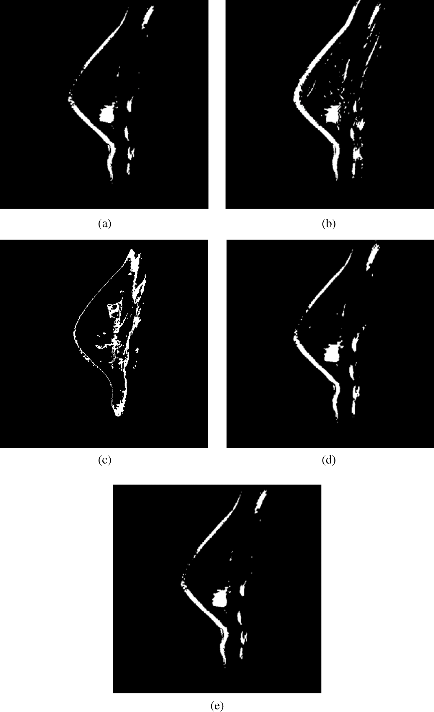

Table 7

Averaged tumor classification rates for ICTA, PCTA, FCM, CEM, and OSP.

Method	Tumor classification rates
	Correct-classification rate (%)	False-alarm rate (%)
Blind source separation method
ICTA	95.78	2.05
PCTA	91.1	2.73
FCM	82.17	11.64
Prior knowledge required method
CEM	98.25	3.02
OSP	80.63	2.46

5.

Conclusion

Although ICA shows good performance in multispectral MRI analysis, it may produce inconsistent results for ICs because ICA uses random initial projection vectors. To solve this problem, we propose a new method called the ICTA for tumor contrast enhancement and segmentation using breast MRIs. ICTA consists of three processes: ICA, ET, and TFR.

After comparison with PCTA, FCM, CEM, OSP, and contrast-injected breast MRIs, our results indicate the possibility of using ICTA for accurate diagnosis. First, ICTA is a BSS method that, unlike CEM or OSP, does not require prior knowledge. Second, the correct IC identification rate by TFR is as high as 92.09%. Third, the tumor region correct-classification rate is as high as 95.78% with a 2.05% false-alarm rate. We anticipate that the high-contrast and binary images generated by ICTA will assist radiologists in breast MRI screening and increase the accuracy of breast tumor diagnosis.