Color correction pipeline optimization for digital cameras

Simone Bianco; Arcangelo R. Bruna; Filippo Naccari; Raimondo Schettini

doi:10.1117/1.JEI.22.2.023014

14 May 2013 Color correction pipeline optimization for digital cameras

Simone Bianco, Arcangelo R. Bruna, Filippo Naccari, Raimondo Schettini

Author Affiliations +

Journal of Electronic Imaging, Vol. 22, Issue 2, 023014 (May 2013). https://doi.org/10.1117/1.JEI.22.2.023014

Abstract

The processing pipeline of a digital camera converts the RAW image acquired by the sensor to a representation of the original scene that should be as faithful as possible. There are mainly two modules responsible for the color-rendering accuracy of a digital camera: the former is the illuminant estimation and correction module, and the latter is the color matrix transformation aimed to adapt the color response of the sensor to a standard color space. These two modules together form what may be called the color correction pipeline. We design and test new color correction pipelines that exploit different illuminant estimation and correction algorithms that are tuned and automatically selected on the basis of the image content. Since the illuminant estimation is an ill-posed problem, illuminant correction is not error-free. An adaptive color matrix transformation module is optimized, taking into account the behavior of the first module in order to alleviate the amplification of color errors. The proposed pipelines are tested on a publicly available dataset of RAW images. Experimental results show that exploiting the cross-talks between the modules of the pipeline can lead to a higher color-rendition accuracy.

1. Introduction

The color rendering accuracy of a digital imaging acquisition device is a key factor to the overall perceived image quality.¹^–³ There are mainly two modules responsible for the color rendering accuracy in a digital camera: the former is the illuminant estimation and correction module, the latter is the color matrix transformation. These two modules together form what may be called the color correction pipeline.

The first stage of the color correction pipeline¹^,³ aims to render the acquired image as closely as possible to what a human observer would have perceived if placed in the original scene, emulating the color constancy feature of the human visual system (HVS), i.e., the ability of perceiving relatively constant colors when objects are lit by different illuminants.⁴ The illuminant estimation is an ill-posed problem,⁵ and it is one of the most delicate modules of the entire image processing pipeline. Numerous methods exist in the literature, and excellent reviews of them can be found in the works of Hordley,⁴ Bianco et al.,⁶ and Gijsenij et al.⁷ A recent research area, which has shown promising results, aims to improve illuminant estimation by using visual information automatically extracted from the images. The existing algorithms exploit both low-level,⁸^,⁹ intermediate-level,¹⁰ and high-level¹¹^,¹² visual information.

The second stage of the color correction pipeline transforms the image data into a standard color space. This transformation, usually called color matrixing, is needed because the spectral sensitivity functions of the sensor color channels rarely match those of the desired output color space. This transformation is usually performed by using a linear transformation matrix, and it is optimized assuming that the illuminant in the scene has been successfully estimated and compensated for Refs. 13 and 14.

Both the illuminant estimation process and the color correction matrix concur in the formation of the overall perceived image quality. These two processes have always been studied and optimized separately, thus ignoring the interactions between them with the only exception (to the best of our knowledge) of the authors that have investigated their interactions and how to optimize them for the overall color accuracy on datasets synthetically generated.⁶ Nevertheless many factors on real systems can affect the color fidelity, e.g., noise, limited dynamic range, and signal degradation due to digital signal processing. This work aims to design and test new and more robust color correction pipelines. The first module exploits different illuminant estimation and correction algorithms that are automatically selected on the basis of the image content. The second module, taking into account the behavior of the first module, makes it possible to alleviate error propagation and improve color rendition accuracy. The proposed pipelines are tested and compared with state of the art solutions on a publicly available dataset of RAW images.¹⁵ Experimental results show that illuminant estimation algorithms exploiting visual information extracted from the images, and taking into account the cross-talks between the modules of the pipeline can significantly improve color rendition accuracy.

2. Image Formation

An image acquired by a digital camera can be represented as a function $ρ$ mainly dependent on three physical factors: the illuminant spectral power distribution $I (λ)$ , the surface spectral reflectance $S (λ)$ , and the sensor spectral sensitivities $C (λ)$ . Using this notation, the sensor responses at the pixel with coordinates $(x, y)$ can be thus described as

Eq. (1)

ρ (x, y) = \int_{ω} I (λ) S (x, y, λ) C (λ) d λ,

where

ω

is the wavelength range of the visible light spectrum,

ρ

and

C (λ)

are three-component vectors. Since the three sensor spectral sensitivities are usually more sensitive, respectively to the low, medium, and high wavelengths, the three-component vector of sensor responses

ρ = (ρ_{1}, ρ_{2}, ρ_{3})

is also referred to as the sensor or camera raw

RGB = (R, G, B)

triplet. In the following, we adopt the convention that RGB triplets are represented by column vectors.

In order to render the acquired image as close as possible to what a human observer would perceive if placed in the original scene, the first stage of the color correction pipeline aims to emulate the color constancy feature of the HVS, i.e., the ability to perceive relatively constant colors when objects are lit by different illuminants. The dedicated module is usually referred to as automatic white balance (AWB), which should be able to determine from the image content the color temperature of the ambient light and compensate for its effects. Numerous methods exist in the literature, and Hordley,⁴ Bianco et al.,⁶ and Gijsenij et al.⁷ give an excellent review of them. Once the color temperature of the ambient light has been estimated, the compensation for its effects is generally based on the Von Kries hypothesis,¹⁶ which states that color constancy is an independent regulation of the three cone signals through three different gain coefficients. This correction can be easily implemented on digital devices as a diagonal matrix multiplication.

The second stage of the color correction pipeline transforms the image data into a standard RGB (e.g., sRGB, ITU-R BT.709) color space. This transformation, usually called color matrixing, is needed because the spectral sensitivity functions of the sensor color channels rarely match those of the desired output color space. Typically this transformation is a $3 \times 3$ matrix with nine variables to be optimally determined, and there are both algebraic¹³ and optimization-based methods¹⁴^,¹⁶ to find it.

The typical color correction pipeline can be thus described as follows:

Eq. (2)

{[\begin{matrix} R \\ G \\ B \end{matrix}]}_{out} = {(α [\begin{matrix} a_{11} & a_{12} & a_{13} \\ a_{21} & a_{22} & a_{23} \\ a_{31} & a_{32} & a_{33} \end{matrix}] [\begin{matrix} r_{awb} \\ g_{awb} \\ b_{awb} \end{matrix}] {[\begin{matrix} R \\ G \\ B \end{matrix}]}_{in})}^{γ},

where

{RGB}_{in}

are the camera raw RGB values,

α

is an exposure compensation common gain, the diagonal matrix

diag (r_{awb}, g_{awb}, b_{awb})

is the channel-independent gain compensation of the illuminant, the full

3 \times 3

matrix

a_{(i, j)}

,

(i, j) = {1, 2, 3}^{2}

is the color space conversion transform from the device-dependent RGB to the sRGB color space,

γ

is the gamma correction defined for the sRGB color space, and

{RGB}_{out}

are the output sRGB values. The exponent

γ

is intended here, with abuse of notation, to be applied to every element of the matrix.

The color correction pipeline is usually composed of a fixed white balance algorithm, coupled with a color matrix transform optimized for a single illuminant.

3. Proposed Approach

In this work, since it has previously been shown⁵ that within a set of AWB algorithms, the best and the worst ones do not exist, but they change on the basis of the image characteristic, we consider a set of single AWB algorithms,¹⁷ and two classification-based modules,¹⁰^,⁸ able to identify the best AWB algorithm to use for each image exploiting automatically extracted information about the image class or image content in terms of low-level features.

For what concerns the matrix transform module, we consider together with a single matrix optimized for a single illuminant a module based on multiple matrices optimized for different illuminants, and we consider matrices optimized taking into account the AWB algorithm behavior.⁶

3.1.

Automatic White Balance Modules

The first AWB module considered is the best single (BS) algorithm extracted from the ones proposed by Van de Weijer et al.¹⁷ They unified a variety of color constancy algorithms in a unique framework. The different algorithms estimate the color $I$ of the illuminant by implementing instantiations of the following equation:

Eq. (3)

I (n, p, σ) = \frac{1}{k} {(\iint \nabla^{n} ρ_{σ} (x, y) |^{p} d x d y)}^{1 / p},

where

n

is the order of the derivative,

p

is the Minkowski norm,

ρ_{σ} (x, y) = ρ_{σ} (x, y) \otimes G_{σ} (x, y)

is the convolution of the image with a Gaussian filter

G_{σ} (x, y)

with scale parameter

σ

, and

k

is a constant to be chosen so that the illuminant color

I

has unit length. Varying the three variables

(n, p, σ)

, it is possible to generate six algorithm instantiations that correspond with well-known and widely used color constancy algorithms. The six different instantiations used in this work are reported in Table 1, together with their underlying assumptions.

Table 1

Color constancy algorithms that can be generated as instantiations of Eq. (3), together with their underlying hypothesis.

Name	( $n$ , $p$ , $σ$ )	Optimized ( $n$ , $p$ , $σ$ )	Assumption
Gray World (GW)	(0, 1, 0)	(0, 1, 0)	Average reflectance in the scene is achromatic
White Point (WP)	(0, $\infty$ , 0)	(0, $\infty$ , 0)	Maximum reflectance in the scene is achromatic
Shades of Gray (SG)	(0, $p$ , 0)	(0, 1.06, 0)	$p$ ’th Minkowski norm of the scene is achromatic
General Gray World (GGW)	(0, $p$ , $σ$ )	(0, 1.08, 0.83)	$p$ ’th Minkowski norm of the scene after local smoothing is achromatic
Gray Edge (GE1)	(1, $p$ , $σ$ )	(1, 1.10, 1.08)	$p$ ’th Minkowski norm of the first order derivative in the scene is achromatic
Second Order Gray Edge (GE2)	(2, $p$ , $σ$ )	(2, 1.55, 1.83)	$p$ ’th Minkowski norm of the second order derivative in the scene is achromatic

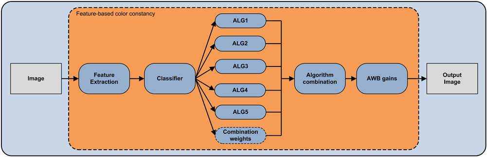
The different AWB instances have been optimized on the dataset proposed by Ciurea and Funt,¹⁸ and the best performing one on an independent training set is selected as the BS algorithm.¹⁰ The optimal parameters found are reported in Table 1.

The second AWB module considered is the class based (CB) algorithm extracted from Ref. 10. It adopts a classification step to assign each image to indoor, outdoor, or ambiguous classes. The classifier, which is described below, is trained on general purpose, low-level features automatically extracted from the images: color histogram, edge direction histogram, statistics on the wavelet coefficients, and color moments (see Ref. 10 for a more detailed description of them). A different AWB algorithm is associated to each of the three possible classes: on the basis of the classification result, only the corresponding AWB algorithm selected is applied. The strategy for the selection and the tuning of the most appropriate algorithm (or combination of algorithms) for each class is fully described.¹⁰ The block diagram of the CB algorithm is reported in Fig. 1.

Fig. 1

Block diagram of the class based (CB) algorithm.

The third module considered is the feature based (FB) algorithm extracted from Ref. 8. It is based on five independent AWB algorithms and a classification step that automatically selects which AWB algorithm to use for each image. It is also possible to use the output of the classifier as weights to combine the estimations of the different algorithms considered.⁵^,¹⁹ The classifier is trained on low-level features automatically extracted from the images. The feature set includes the general purpose features used for the CB algorithm and some features specifically designed. These features are the number of different colors, the percentage of color components that are clipped to the highest and lowest value that can be represented in the image color space, the magnitudes of the edges, and a cast index representing the extent of the presence of a color cast in the image (inspired by the work done in Ref. 20). See Ref. 8 for a detailed description of the features. The block diagram of the FB algorithm is reported in Fig. 2.

Fig. 2

Block diagram of the feature based (FB) algorithm.

The CB and FB AWB modules share the same classification strategy. They use tree classifiers constructed according to the CART methodology.²¹ Briefly, tree classifiers are classifiers produced by recursively partitioning the predictors space, each split being formed by conditions related to the predictors values. In tree terminology, subsets are called nodes: the predictors space is the root node, terminal subsets are terminal nodes, and so on. Once a tree has been constructed, a class is assigned to each of the terminal nodes, and when a new case is processed by the tree, its predicted class is the class associated with the terminal node into which the case finally moves on the basis of its predictors values. The construction process is based on training sets of cases of known class. Tree classifiers compare well with other consolidated classifiers. Many simulation studies have shown their accuracy to be very good, often close to the achievable optimum.²¹ Moreover, they provide a clear understanding of the conditions that drive the classification process. Finally, they imply no distributional assumptions for the predictors and can handle both quantitative and qualitative predictors in a natural way. Since in high dimensional and complex problems, as is the case here, it is practically impossible to obtain in one step good results in terms of accuracy, no matter how powerful the chosen class of classifiers is, we decided to perform the classification by also using what is called a “perturbing and combining” method.²²^,²³ Methods of this kind, which generate in various ways multiple versions of a base classifier and use these to derive an aggregate classifier, have proved successful in improving accuracy. We used bagging (bootstrap aggregating), since it is particularly effective when the classifiers are unstable, as trees are; that is, when small perturbations in the training sets, or in the construction process of the classifiers, may result in significant changes in the resulting prediction. With bagging the multiple versions of the base classifier are formed by making bootstrap replicates of the training set and using them as new training sets. The aggregation is made by majority vote. In any particular bootstrap replicate, each element of the training set may appear repeated, or not at all, since the replicates are obtained by resampling with replacement. To provide a measure of confidence in the classification results and, still, greater accuracy, we applied an ambiguity rejection rule²⁴ to the bagged classifier: the classification obtained by means of the majority vote is rejected if the percentage of trees that contribute to it is lower than a given threshold. In this way only those results to which the classifier assigns a given confidence, as set by the threshold, are accepted.

3.2.

Color Matrix Transform Modules

The color matrix transform modules considered are extracted from the strategies proposed by the authors in Ref. 6. In the following a more compact version of Eq. (2) is used:

Eq. (4)

{RGB}_{out} = {(α {AI}_{W} \cdot {RGB}_{in})}^{γ},

where

α

,

I_{W}

and

A

, respectively represent the exposure compensation gain, the diagonal matrix for the illuminant compensation and the color matrix transformation.

The first color matrix transform module considered is named Single ILLuminant (SILL) since it is based on a single matrix transform optimized for a single illuminant. Given a set of $n$ different patches whose sRGB values $r$ are known, and the corresponding camera raw values $c$ measured by the sensor when the patches are lit by the chosen illuminant, what is usually done is to find the matrix $M$ that satisfies

Eq. (5)

M = \arg (\min_{A \in R^{3 \times 3}} \sum_{k = 1}^{n} E (r_{k}, {(α {AI}_{W} c_{k})}^{γ})),

where

E (\cdot)

is the chosen error metric, and the subscript

k

indicates the triplet in the

k

’th column of the matrix, i.e., it indicates the tri-chromatic values of the

k

’th patch. In this work, the error metric

E

adopted is the average

Δ E_{94}

colorimetric error between the reference and calculated sRGB values mapped in the CIEL*a*b* color space. The values of

α

and

I_{W}

have been previously computed in order to perfectly expose the scene and compensate for the illuminant. Given the importance of neutral tones in the color reproduction, the 9 deg of freedom of the color matrix transformation are usually reduced to six by a white point preserving constraint, i.e., a neutral color in the device-dependent color space should be mapped to a neutral color in the device independent color space. This can be easily obtained by constraining each row to sum to one.

The second color matrix transform module considered is named multiple illuminant (MILL). It differs from the first module since it is based on multiple matrix transforms, with each one optimized for a different illuminant by using Eq. (5). Therefore for each image a different matrix transform is used. First of all the AWB algorithm is applied to estimate the illuminant compensation gains, then the two training illuminants ${ILL}_{i}$ and ${ILL}_{j}$ with the most similar gains are identified, and the matrix transform is calculated as follows:

Eq. (6)

M = α M_{{ILL}_{i}} + (1 - α) M_{{ILL}_{j}},

where

Eq. (7)

α = \frac{D (gains, {gains}_{j})}{D (gains, {gains}_{i}) + D (gains, {gains}_{j})},

and

D

is the angular error between the gains considered, i.e.,

Eq. (8)

D = \arccos (\frac{{gains}_{1}^{T} \cdot {gains}_{2}}{‖ {gains}_{1} ‖ \cdot ‖ {gains}_{2} ‖}) .

The reference illuminants could be a set of predefined standard illuminants (as done in Ref. 6), or it could be found by clustering the ground truth illuminants of the images in the training set. Then, for each centroid of the clusters found, the best color correction matrix is computed. The latter approach is here adopted as described in Sec. 5.

The third color matrix transform module considered is named SILL with white balance error buffer (SILLWEB). It is based on a single matrix transform optimized for a single illuminant, taking into account the behavior of the AWB module used. Suppose the best gain coefficients $g_{0} = [r_{0}, g_{0}, b_{0}]$ have already been determined and reshaped in the diagonal transform $G_{0}$ to compensate the considered illuminant; we then generate a set $g = {g_{1}, \dots, g_{s}}$ of $s$ gain coefficients with different distances from $g_{0}$ , measured using the $Δ E_{94}$ error metric. These can be used to simulate errors that may occur in the AWB process and are paired with a weights distribution $u = {u_{0}, \dots, u_{s}}$ that reflects the frequency of the considered errors. The optimization problem can be thus formulated as

Eq. (9)

M = \arg (\min_{A \in R^{3 \times 3}} \sum_{j = 0}^{s} u_{j} (\sum_{k = 1}^{n} E (r_{k}, {(α_{j} {AG}_{j} c_{k})}^{γ}))) subject to \sum_{j = 1}^{3} A_{(i, j)} = 1, \forall i \in {1, 2, 3},

where

G_{j}

,

j = {0, \dots, s}

are the diagonal matrices obtained, respectively, by reshaping the gain coefficients

{g_{0}, \dots, g_{s}}

.

The fourth color matrix transform module considered is named MILL with white balance error buffer (MILLWEB). It differs from the third module since it is based on multiple matrix transforms, with each one optimized for a different taking illuminant using Eq. (9). For each image a different matrix transform is used. First the AWB algorithm is applied to estimate the illuminant compensation gains, then the two training illuminants ${ILL}_{i}$ and ${ILL}_{j}$ with the most similar gains are identified, and the matrix transform is calculated as in Eqs. (6) and (7).

All the matrices for the different color matrix transform modules are found by optimization using the pattern search method (PSM). PSMs are a class of direct search methods for nonlinear optimization.²⁵ PSMs are simple to implement and do not require any explicit estimate of derivatives. Furthermore, global convergence can be established under certain regularity assumptions of the function to minimize.²⁶

The general form of a PSM is reported in Table 2, where $f$ is the function to be minimized, $k$ is the iteration number, $x_{k}$ is the current best solution, $D_{k}$ is the set of search directions, and $Δ_{k}$ is a step-length parameter.

Table 2

Pseudo-code of the general form of a pattern search method (PSM).

WHILE $Δ_{k} >$ thresh and $k <$ maximum iteration number

FOR each $d_{k} \in D_{k}$

x^{+} = x_{k} + Δ_{k} d_{k}

IF

\exists d_{k} \in D_{k} : f (x^{+}) < f (x_{k})

THEN

x_{k + 1} = x^{+}

Δ_{k + 1} = α_{k} Δ_{k}

with

α_{k} > 1

ELSE

x_{k + 1} = x_{k}

Δ_{k + 1} = β_{k} Δ_{k}

with

β_{k} < 1

ENDIF

ENDFOR

k = k + 1

ENDWHILE

4. Experimental Setup

The aim of this section is to investigate how the proposed methods can be combined in order to design a new color correction pipeline. In particular, we investigate the color accuracy improvement that the illuminant estimation algorithms of Sec. 3 and the color space conversion strategies of Sec. 4 can give when they are used individually and combined properly.

4.1.

Image Dataset and Evaluation Procedure

To test the performance of the investigated processing pipelines, a standard dataset of RAW camera images having a known color target is used.¹⁵ This dataset is captured using a high-quality digital SLR camera in RAW format and is therefore free of any color correction. This dataset was originally available in sRGB-format, but Shi and Funt²⁷ reprocessed the raw data to obtain linear images with a higher dynamic range (12 bits as opposed to standard 8 bits). The dataset consists of a total of 568 images. The Macbeth ColorChecker (MCC) chart is included in every scene acquired, and this allows us to estimate accurately the actual illuminant of each acquired image.²⁷ Some examples from the image dataset are shown in Fig. 3. The spatial coordinates of the MCC in each image of the dataset have been automatically detected²⁸ and manually refined.

Fig. 3

Typical examples of the images belonging to the RAW dataset used.

The flowchart of the evaluation procedure adopted is given in Fig. 4, where it can be seen that the only step in which the MCC chart is cropped is the illuminant estimation one.

Fig. 4

Pipeline evaluation: the Macbeth ColorChecker (MCC) is localized and masked; the illuminant is estimated on the image with the masked MCC, and the unmasked image is illuminant-corrected on the basis of this estimate; the color correction matrix is then applied to this image, the RGB coordinates of the MCC are extracted and compared with the MCC theoretical ones.

The investigated illuminant estimation algorithms described in Sec. 3 have been individually applied to the images of the dataset, excluding the MCC chart regions that have been previously cropped. Given these estimations, the illuminant corrections are then performed on the whole images (therefore also including the MCC chart).

The color matrix transformations found according to the computational strategies described in Sec. 4 are then applied to the whole, white balanced images. For each processed image, the MCC chart is then extracted, and the average RGB values of the central area of each patch are calculated. The color rendition accuracy of the pipeline is measured in terms of average $Δ E_{94}$ error between the CIEL*a*b* color coordinates of the color corrected MCC patches, and their theoretical CIEL*a*b* values that are computed using standard equations from their theoretical RGB values.

5. Pipeline Training and Testing

In this section the color correction pipelines composed of the combination of the modules for the illuminant estimation algorithms of Sec. 3 and the color matrix transform modules of Sec. 4 are tested. Globally, 20 different pipelines have been tested; they are generated as an exhaustive combination of the modules proposed. The acronyms of the proposed strategies are generated using the scheme reported in Fig. 5.

Fig. 5

Composition rules for the generation of the acronyms of the strategies compared.

The first part indicates the typology of AWB used ( $BS = Best Single$ : the BS AWB algorithm among the general purpose ones considered in Ref. 10 is used; $CB = Class - Based$ : the algorithm described in Ref. 10, based on an indoor-outdoor classification is used; $FB = Feature - Based$ : the algorithm described in Ref. 8 is used, which is based on five independent AWB algorithms and a classification step that automatically selects which AWB algorithm to use for each image). The second part indicates the number and type of the color correction matrix used ( $SILL = s ingle ill uminant$ : single matrix optimized for a fixed single illuminant, $MILL = m ultiple ill uminant$ : multiple matrices each optimized for a different single illuminant). The third part indicates if the strategy implements color correction matrices able to compensate for AWB errors ( $WEB = White balance Error Buffer$ ) or not (0). The last part indicates if a real classifier has been used in the AWB module (0) or manual classification (ideal). The symbol 0 is reported in the scheme but is intended as the null character and thus omitted in the acronyms generated.

Since the considered modules need a training phase, 30% of the images in the dataset were randomly selected and used as training set; the remaining 70% were used as test set. For the strategies that are based on multiple color correction matrices, these are computed by first clustering the ground truth illuminants of the images in the training set into seven different clusters using a $k$ -means algorithm.²⁹ Then, for each centroid of the clusters found, the best color correction matrix is calculated.

6. Experimental Results

The average over the test images of the average $Δ E_{94}$ colorimetric errors obtained by the tested pipelines on the MCCs are computed and reported in Table 3. The average of the maximum $Δ E_{94}$ colorimetric error are also reported. For both the error statistics the percentage improvement over the baseline method, i.e., BS-SILL pipeline, are reported. The results of the pipelines tested are clustered into four different groups depending on the color correction strategy adopted.

Table 3

Color correction pipeline accuracy comparison.

Pipeline	Average $Δ E_{94}$	Improvement	Average maximum $Δ E_{94}$	Improvement
BS-SILL	7.5309	-.--%	20.5952	-.--%
$CB - {SILL}_{ideal}$	7.3875	1.90%	20.4129	0.89%
CB-SILL	7.5541	$- 0.31 %$	20.5338	0.30%
$FB - {SILL}_{ideal}$	6.5324	13.26%	17.9495	12.85%
FB-SILL	7.3684	2.16%	18.9716	7.88%
BS-MILL	6.9636	7.53%	19.9529	3.12%
$CB - {MILL}_{ideal}$	6.5930	12.45%	17.8758	13.20%
CB-MILL	6.8954	8.43%	18.4612	10.36%
$FB - {MILL}_{ideal}$	5.9695	20.73%	16.8695	18.09%
FB-MILL	6.7199	10.77%	18.8840	8.31%
BS-SILLWEB	6.8079	9.60%	18.4964	10.19%
$CB - {SILLWEB}_{ideal}$	6.3627	15.51%	17.5217	14.92%
CB-SILLWEB	6.6753	11.36%	18.0941	12.14%
$FB - {SILLWEB}_{ideal}$	5.8362	22.50%	15.8122	23.22%
FB-SILLWEB	6.4811	13.94%	18.5985	9.69%
BS-MILLWEB	6.4654	14.15%	17.6920	14.09%
$CB - {MILLW}_{ideal}$	6.2949	16.41%	16.8606	18.13%
CB-MILLWEB	6.4058	14.94%	17.2316	16.33%
$FB - {MILLWEB}_{ideal}$	5.3232	29.32%	14.3284	30.43%
FB-MILLWEB	6.1368	18.51%	16.6687	19.07%

To understand if the differences in performance among the pipelines considered are statistically significant, we have used the Wilcoxon signed-rank test.³⁰ This statistical test permits comparison of the whole error distributions without limiting to punctual statistics. Furthermore, it is well suited because it does not make any assumptions about the underlying error distributions, and it is easy to find, using for example the Lilliefors test,³¹ that the assumption about the normality of the error distributions does not always hold. Let $X$ and $Y$ be random variables representing the $Δ E_{94}$ errors obtained on the MCCs of all test images by two different pipelines. Let $μ_{X}$ and $μ_{Y}$ be the median values of such random variables. The Wilcoxon signed-rank test can be used to test the null hypothesis $H_{0} : μ_{X} = μ_{Y}$ against the alternative hypothesis $H_{1} : μ_{X} \neq μ_{Y}$ . We can test $H_{0}$ against $H_{1}$ at a given significance level $α$ . We reject $H_{0}$ and accept $H_{1}$ if the probability of observing the error differences we obtained is less than or equal to $α$ . We have used the alternative hypothesis $H_{1} : μ_{X} < μ_{Y}$ with a significance level $α = 0.05$ . Comparing the error distributions of each pipeline with all the others gives the results reported in Table 4. A “+” sign in the $(i, j)$ position of the table means that the error distribution obtained with the pipeline $i$ has been considered statistically better than that obtained with the pipeline $j$ ; a “−” sign that it has been considered statistically worse, and a “=“ sign that they have been considered statistically equivalent.

Table 4

Wilcoxon signed rank test results on the error distributions obtained by the different pipelines. A “+” sign in the (i, j)-position means that the error distribution obtained with the pipeline i has been considered statistically better than that obtained with the pipeline j, a “−” sign that it has been considered statistically worse, and an “=” sign that they have been considered statistically equivalent.

ID	Pipeline	1	2	3	4	5	6	7	8	9	10	11	12	13	14	15	16	17	18	19	20	Score
1	BS-SILL	=	−	=	−	−	−	−	−	−	−	−	−	−	−	−	−	−	−	−	−	0
2	$CB - {SILL}_{ideal}$	+	=	+	−	=	−	−	−	−	−	−	−	−	−	−	−	−	−	−	−	2
3	CB-SILL	=	−	=	−	−	−	−	−	−	−	−	−	−	−	−	−	−	−	−	−	0
4	$FB - {SILL}_{ideal}$	+	+	+	=	+	+	=	+	−	+	+	−	+	−	−	−	−	−	−	−	9
5	FB-SILL	+	=	+	−	=	−	−	−	−	−	−	−	−	−	−	−	−	−	−	−	2
6	BS-MILL	+	+	+	−	+	=	−	−	−	−	−	−	−	−	−	−	−	−	−	−	4
7	$CB - {MILL}_{ideal}$	+	+	+	=	+	+	=	+	−	+	+	−	+	−	−	−	−	−	−	−	9
8	CB-MILL	+	+	+	−	+	−	−	=	−	−	+	−	−	−	−	−	−	−	−	−	5
9	$FB - {MILL}_{ideal}$	+	+	+	+	+	+	+	+	=	+	+	+	+	−	+	+	+	+	−	+	17
10	FB-MILL	+	+	+	−	+	+	−	+	−	=	+	−	−	−	−	−	−	−	−	−	7
11	BS-SILLWEB	+	+	+	−	+	+	−	+	−	−	=	−	−	−	−	−	−	−	−	−	6
12	$CB - {SILLWEB}_{ideal}$	+	+	+	+	+	+	+	+	−	+	+	=	+	−	+	+	−	=	−	−	13
13	CB-SILLWEB	+	+	+	−	+	+	−	+	−	+	+	−	=	−	−	−	−	−	−	−	8
14	$FB - {SILLWEB}_{ideal}$	+	+	+	+	+	+	+	+	+	+	+	+	+	=	+	+	+	+	−	+	18
15	FB-SILLWEB	+	+	+	+	+	+	+	+	−	+	+	−	+	−	=	=	−	−	−	−	11
16	BS- MILLWEB	+	+	+	+	+	+	+	+	−	+	+	−	+	−	=	=	−	−	−	−	11
17	$CB - {MILLWEB}_{ideal}$	+	+	+	+	+	+	+	+	−	+	+	+	+	−	+	+	=	+	−	−	15
18	CB-MILLWEB	+	+	+	+	+	+	+	+	−	+	+	=	+	−	+	+	−	=	−	−	13
19	$FB - {MILLWEB}_{ideal}$	+	+	+	+	+	+	+	+	+	+	+	+	+	+	+	+	+	+	=	+	19
20	FB-MILLWEB	+	+	+	+	+	+	+	+	−	+	+	+	+	−	+	+	+	+	−	=	16

It is possible to note in Table 3 that in all the groups of pipelines proposed (groups that share the same color correction matrix strategy, i.e., SILL, MILL, SILLWEB, and MILLWEB), the use of the FB AWB leads to a higher color-rendition accuracy with respect to the use of the CB AWB and of the BS AWB. It is interesting to notice that significant improvements in the color rendition accuracy can be achieved even if the classifiers used for the feature and CB AWB strategies are not optimal.

Analyzing the behavior of the pipelines sharing the same AWB strategy, it is possible to notice that the results of Ref. 6 are also confirmed. In fact, the multiple illuminant color correction (MILL) performs better than the single illuminant one (SILL). The single illuminant color correction, which is optimized taking into account the statistics of how the AWB algorithm tends to make errors (SILLWEB), performs better than the multiple illuminant color correction (MILL). Finally, the multiple illuminant color correction with white balance error buffer (MILLWEB) performs better than the corresponding single illuminant instantiation (SILLWEB).

For what concerns the best pipeline proposed, which is the FB-MILLWEB, it can be observed that when using the ideal classifier, 48% of improvement (from 0% to 14.15% with respect to the benchmarking pipeline) is due to the use of the MILLWEB color correction matrix approach and the remaining 52% (from 14.15% to 29.32% with respect to the benchmarking pipeline) to the FB AWB approach. When using the real classifier the remaining part to the FB AWB approach. This can be considered a lower bound of the pipeline performance, since, as already explained before, the classifier used is not optimal for the image database used.

In Fig. 6 the workflow of the best performing pipeline proposed, i.e., the FB-MILLWEB, is reported. The low-level features considered are extracted from the RAW image and fed to the classifier, which as output gives the weights to use for the linear combination of the five simple AWB algorithms considered. The AWB correction gains given by the five simple AWB algorithms considered are then combined to give the AWB correction gains to use. The image is then corrected with these gains to obtain an AWB corrected image. The correction gains are used to identify the two training illuminants most similar to the estimated one. The two color correction matrices computed for the two identified illuminants are retrieved and combined accordingly to the illuminant similarity. The image is finally color corrected using this color correction matrix.

Fig. 6

Workflow of the pipeline composed of the feature-based (FB) automatic white balance (AWB) and the multiple illuminant color matrixing with white balance error buffer (FB-MILLWEB).

In Fig. 7 it is shown the image on which the best pipeline proposed, i.e., FB-MILLWEB, makes the larger color error. For sake of comparison, the results obtained with BS-SILL (a); FB-SILL (b); FB-SILLWEB (c); and FB-MILLWEB (d) pipelines are also shown. Finally in Fig. 7(e) the best achievable results is reported, which is computed using the achromatic patches of the MCC to estimate the ideal AWB gains, and the color space transformation has been optimized specifically for this image. Taking into account that the image reproduction may have altered the image content, making the differences between the different pipelines not clearly appreciable, we report in Fig. 8 the error distribution between the ideal color-corrected image [Fig. 7(e)] and the output of the tested pipelines. The images reported in Fig. 7(a)–7(d) are therefore converted in CIEL*a*b* color coordinates and the $Δ E_{94}$ colorimetric error is computed for every pixel of each image with respect to the ideal image. The histograms of the colorimetric errors are, respectively reported in Fig. 8(a)–8(d). To compare the color error distributions of the pipelines considered on this image, we use the Wilcoxon signed-rank test. The output of the test is reported in Table 5. It is possible to notice that even in the worst case example, the FB-MILLWEB pipeline, which is the best on the whole dataset, is still the best one.

Fig. 7

Worst case example. The results obtained by different pipelines are reported: BS-SILL (a); FB-SILL (b); FB-SILLWEB (c); FB-MILLWEB (d); and ideal correction (e).

Fig. 8

Histograms of the $Δ E_{94}$ colorimetric error for the images reported in Figs. 7(a)–(d), using Figs. 7(e) as reference.

Table 5

Wilcoxon signed rank test results on the error distributions obtained by the different pipelines on the worst case example.

ID	Pipeline	1	2	3	4	Score
1	BS-SILL	=	−	−	−	0
2	FB-SILL	+	=	−	−	1
3	FB-SILLWEB	+	+	=	−	2
4	FB-MILLWEB	+	+	+	=	3

7. Conclusion

Digital camera sensors are not perfect and do not encode colors the same way in which the human eye does. A processing pipeline is thus needed to convert the RAW image acquired by the camera to a representation of the original scene that should be as faithful as possible. In this work we have designed and tested new color correction pipelines, which exploit the cross-talks between its modules in order to lead to a higher color rendition accuracy. The effectiveness of the proposed pipelines is shown on a publicly available dataset of RAW images. The experimental results show that in all the groups of pipelines proposed (groups that share the same color correction matrix strategy, i.e., SILL, MILL, SILLWEB, and MILLWEB), the use of the FB AWB leads to a higher color-rendition accuracy when compared with the use of the CB AWB and of the BS AWB. It is interesting to note that significant improvements in the color-rendition accuracy can be achieved even if the classifiers used for the feature and CB AWB strategies are not optimal. Analyzing the behavior of the pipelines sharing the same AWB strategy, it is possible to note that the results of Ref. 6 are also confirmed. In fact the multiple illuminant color correction (MILL) performs better than the single illuminant one (SILL). The single illuminant color correction, which is optimized taking into account the statistics of how the AWB algorithm tends to make errors (SILLWEB), performs better than the multiple illuminant color correction (MILL). Finally, the multiple illuminant color correction with white balance error buffer (MILLWEB) performs better than the corresponding single illuminant instantiation (SILLWEB).

The present work makes it also possible to identify some open issues that must be addressed in the future. Illuminant estimation algorithms are generally based on the simplifying assumption that the spectral distribution of a light source is uniform across scenes. However, in reality, this assumption is often violated due to the presence of multiple light sources.³² Some multiple illuminant estimation algorithms have been proposed;³³ however, they assume very simple setups, or a knowledge of the number and color of the illuminants.³⁴

Once the scene illuminant has been estimated, the scene is usually corrected in the RGB device dependent color space using the diagonal Von Kries model.¹⁶ Several studies have investigated the use of different color spaces for the illuminant correction³⁵^,³⁶ as well as nondiagonal models.³⁷ A different approach could be to use chromatic adaptation transforms³⁸^,³⁹ to correct the scene illuminant.

As suggested by a reviewer, the use of larger color correction matrices should be investigated, taking into account not only color rendition accuracy, but also noise amplification in particular on dark colors.

References

1.

R. Ramanathet al., “Color image processing pipeline,” IEEE Signal Proc. Mag., 22 (1), 34 –43 (2005). http://dx.doi.org/10.1109/MSP.2005.1407713 ISPRE6 1053-5888 Google Scholar

2.

C. Weerasingheet al., “Novel color processing architecture for digital cameras with CMOS image sensors,” IEEE Trans. Consum. Electron., 51 (4), 1092 –1098 (2005). http://dx.doi.org/10.1109/TCE.2005.1561829 ITCEDA 0098-3063 Google Scholar

3.

W.-C. Kaoet al., “Design consideration of color image processing pipeline for digital cameras,” IEEE Trans. Consum. Electron., 52 (4), 1144 –1152 (2006). http://dx.doi.org/10.1109/TCE.2006.273126 ITCEDA 0098-3063 Google Scholar

4.

S. D. Hordley, “Scene illuminant estimation: past, present, and future,” Color Res. Appl., 31 (4), 303 –314 (2006). http://dx.doi.org/10.1002/(ISSN)1520-6378 CREADU 0361-2317 Google Scholar

5.

S. BiancoF. GaspariniR. Schettini, “Consensus based framework for illuminant chromaticity estimation,” J. Electron. Imag., 17 (2), 023013 (2008). http://dx.doi.org/10.1117/1.2921013 JEIME5 1017-9909 Google Scholar

6.

S. Biancoet al., “Color space transformations for digital photography exploiting information about the illuminant estimation process,” J. Opt. Soc. Am. A, 29 (3), 374 –384 (2012). http://dx.doi.org/10.1364/JOSAA.29.000374 JOAOD6 0740-3232 Google Scholar

7.

A. GijsenijT. GeversJ. van de Weijer, “Computational color constancy: survey and experiments,” IEEE Trans. Image Proc., 20 (9), 2475 –2489 (2011). http://dx.doi.org/10.1109/TIP.2011.2118224 IIPRE4 1057-7149 Google Scholar

8.

S. Biancoet al., “Automatic color constancy algorithm selection and combination,” Pattern Recogn., 43 (3), 695 –705 (2010). http://dx.doi.org/10.1016/j.patcog.2009.08.007 PTNRA8 0031-3203 Google Scholar

9.

A. GijsenijT. Gevers, “Color constancy using natural image statistics and scene semantics,” IEEE Trans. Pattern Anal. Mach. Intell., 33 (4), 687 –698 (2011). http://dx.doi.org/10.1109/TPAMI.2010.93 ITPIDJ 0162-8828 Google Scholar

10.

S. Biancoet al., “Improving color constancy using indoor-outdoor image classification,” IEEE Trans. Image Proc., 17 (12), 2381 –2392 (2008). http://dx.doi.org/10.1109/TIP.2008.2006661 IIPRE4 1057-7149 Google Scholar

11.

J. van de WeijerC. SchmidJ. Verbeek, “Using high-level visual information for color constancy,” in Proc. IEEE 14th Int. Conf. on Computer Vision, 1 –8 (2007). Google Scholar

12.

S. BiancoR. Schettini, “Color constancy using faces,” in Proc. IEEE Conf. Computer Vision and Pattern Recognit., 65 –72 (2012). Google Scholar

13.

P. M. Hubelet al., “Matrix calculations for digital photography,” in Proc. 5th Color Imaging Conf.: Color Science, Systems and Applications, 105 –111 (1997). Google Scholar

14.

S. Biancoet al., “A new method for RGB to XYZ transformation based on pattern search optimization,” IEEE Trans. Consum. Electron., 53 (3), 1020 –1028 (2007). http://dx.doi.org/10.1109/TCE.2007.4341581 ITCEDA 0098-3063 Google Scholar

15.

P. V. Gehleret al., “Bayesian color constancy revisited,” in Proc. IEEE Computer Society Conf. on Computer Vision and Pattern Recognit., 1 –8 (2008). Google Scholar

16.

J. von Kries, Chromatic Adaptation, Festschrift der Albrecht-Ludwig-Universitat, Fribourg (1902). Google Scholar D. L. MacAdam, Sources of Color Science, MIT Press, Cambridge (1970). Google Scholar

17.

J. van de WeijerT. GeversA. Gijsenij, “Edge-based color constancy,” IEEE Trans. Image Proc., 16 (9), 2207 –2214 (2007). http://dx.doi.org/10.1109/TIP.2007.901808 IIPRE4 1057-7149 Google Scholar

18.

F. CiureaB. Funt, “A large image database for color constancy research,” in Proc. IS&T/SID 11th Color Imaging Conf., 160 –164 (2003). Google Scholar

19.

S. BiancoF. GaspariniR. Schettini, “Combining strategies for white balance,” Proc. SPIE, 6502 65020D (2007). http://dx.doi.org/10.1117/12.705190 PSISDG 0277-786X Google Scholar

20.

F. GaspariniR. Schettini, “Color balancing of digital photos using simple image statistics,” Pattern Recogn., 37 (6), 1201 –1217 (2004). http://dx.doi.org/10.1016/j.patcog.2003.12.007 PTNRA8 0031-3203 Google Scholar

21.

L. Breimanet al., Classification and Regression Trees, Wadsworth and Brooks/Cole, Belmont, California (1984). Google Scholar

22.

L. Breiman, “Bagging predictors,” Mach. Learn., 26 (2), 123 –140 (1996). MALEEZ 0885-6125 Google Scholar

23.

L. Breiman, “Arcing classifiers,” Ann. Stat., 26 (3), 801 –849 (1998). http://dx.doi.org/10.1214/aos/1024691079 ASTSC7 0090-5364 Google Scholar

24.

A. VailayaA. Jain, “Reject option for VQ-based Bayesian classification,” in Proc. 15th Int. Conf. Pattern Recognit., 48 –51 (2000). Google Scholar

25.

R. M. LewisV. Torczon, “Pattern search methods for linearly constrained minimization,” SIAM J. Optim., 10 (3), 917 –941 (2000). http://dx.doi.org/10.1137/S1052623497331373 SJOPE8 1095-7189 Google Scholar

26.

R. M. LewisV. Torczon, “On the convergence of pattern search algorithms,” SIAM J. Optim, 7 (1), 1 –25 (1997). http://dx.doi.org/10.1137/S1052623493250780 SJOPE8 1095-7189 Google Scholar

27.

L. ShiB. V. Funt, (2012) http://www.cs.sfu.ca/colour/data/ July ). 2012). Google Scholar

28.

S. BiancoC. Cusano, “Color target localization under varying illumination conditions,” in Proc. 3rd Int. Workshop on Computational Color Imaging, 245 –255 (2011). Google Scholar

29.

J. A. HartiganM. A. Wong, “Algorithm AS136: A k-means clustering algorithm,” Appl. Stat., 28 100 –108 (1979). http://dx.doi.org/10.2307/2346830 Google Scholar

30.

F. Wilcoxon, “Individual comparisons by ranking methods,” Biometrics, 1 (6), 80 –83 (1945). http://dx.doi.org/10.2307/3001968 BIOMB6 0006-341X Google Scholar

31.

H. Lilliefors, “On the Kolmogorov-Smirnov test for normality with mean and variance unknown,” J. Am. Stat. Assoc., 62 (318), 399 –402 (1967). http://dx.doi.org/10.1080/01621459.1967.10482916 JSTNAL 0003-1291 Google Scholar

32.

A. GijsenijR. LuT. Gevers, “Color constancy for multiple light sources,” IEEE Trans. Image Proc., 21 (2), 697 –707 (2012). http://dx.doi.org/10.1109/TIP.2011.2165219 IIPRE4 1057-7149 Google Scholar

33.

M. Ebner, Color Constancy, John Wiley & Sons, England (2007). Google Scholar

34.

E. Hsuet al., “Light mixture estimation for spatially varying white balance,” in Proc. ACM SIGGRAPH, (2008). Google Scholar

35.

K. BarnardF. CiureaB. Funt, “Sensor sharpening for computational color constancy,” J. Opt. Soc. Am. A, 18 (11), 2728 –2743 (2001). http://dx.doi.org/10.1364/JOSAA.18.002728 JOAOD6 0740-3232 Google Scholar

36.

F. Xiaoet al., “Preferred color spaces for white balancing,” Proc. SPIE, 5017 342 –350 (2003). http://dx.doi.org/10.1117/12.478482 PSISDG 0277-786X Google Scholar

37.

B. FuntH. Jiang, “Nondiagonal color correction,” in Proc. Int. Conf. Image Process., 481 –484 (2003). Google Scholar

38.

“A review of chromatic adaptation transforms,” (2004). Google Scholar

39.

S. BiancoR. Schettini, “Two new von Kries based chromatic adaptation transforms found by numerical optimization,” Color Res. App., 35 (3), 184 –192 (2010). http://dx.doi.org/10.1002/col.v35:3 CREADU 0361-2317 Google Scholar

Biography

Simone Bianco obtained a PhD in computer science at DISCo (Dipartimento di Informatica, Sistemistica e Comunicazione) of the University of Milano-Bicocca, Italy, in 2010. He obtained BSc and the MSc degrees in mathematics from the University of Milano-Bicocca, Italy, respectively, in 2003 and 2006. He is currently a postdoc working on image processing. The main topics of his current research concern digital still cameras processing pipelines, color space conversions, optimization techniques, and characterization of imaging devices.

Arcangelo R. Bruna received a master’s degree from Palermo University, Italy, in 1998. He works for ST Microelectronics, and his research interests are in the area of image processing (noise reduction, auto white balance, video stabilization, etc.) and computer vision algorithms (visual search). He is also currently involved in the MPEG-CDVS (compact descriptors for visual search) standardization.

Filippo Naccari received his MS Italian degree in electronic engineering at University of Palermo, Italy. Since July 2002, he has been working at STMicroelectronics as researcher at the Advanced System Technology, Computer Vision Group, Catania Lab, Italy. His research interests are in the field of digital color and image processing, color constancy, and digital images coding.

Raimondo Schettini is a professor at the University of Milano Bicocca (Italy). He is vice director of the Department of Informatics, Systems and Communication, and head of Imaging and Vision Lab ( www.ivl.disco.unimib.it). He has been associated with Italian National Research Council (CNR) since 1987 where he has headed the Color Imaging lab from 1990 to 2002. He has been team leader in several research projects and published more than 250 reference papers and six patents about color reproduction and image processing, analysis, and classification. He has been recently elected fellow of the International Association of Pattern Recognition (IAPR) for his contributions to pattern recognition research and color image analysis.

© The Authors. Published by SPIE under a Creative Commons Attribution 3.0 Unported License. Distribution or reproduction of this work in whole or in part requires full attribution of the original publication, including its DOI.

Citation Download Citation

Simone Bianco, Arcangelo R. Bruna, Filippo Naccari, and Raimondo Schettini "Color correction pipeline optimization for digital cameras," Journal of Electronic Imaging 22(2), 023014 (14 May 2013). https://doi.org/10.1117/1.JEI.22.2.023014

Published: 14 May 2013

Access the abstract

JOURNAL ARTICLE
11 PAGES

DOWNLOAD PAPER SAVE TO MY LIBRARY

GET CITATION

CITATIONS

Cited by 34 scholarly publications and 1 patent.

Explore citations on Lens.org

RIGHTS & PERMISSIONS

Get copyright permission Get copyright permission on Copyright Marketplace

KEYWORDS

Transform theory

Digital cameras

Error analysis

RGB color model

Sensors

Image processing

Matrices

1.

Introduction

2.

Image Formation

Eq. (1)

Eq. (2)

3.

Proposed Approach

3.1.

Automatic White Balance Modules

Eq. (3)

Table 1

Fig. 1

Fig. 2

3.2.

Color Matrix Transform Modules

Eq. (4)

Eq. (5)

Eq. (6)

Eq. (7)

Eq. (8)

Eq. (9)

Table 2

4.

Experimental Setup

4.1.

Image Dataset and Evaluation Procedure

Fig. 3

Fig. 4

5.

Pipeline Training and Testing

Fig. 5

6.

Experimental Results

Table 3

Table 4

Fig. 6

Fig. 7

Fig. 8

Table 5

7.

Conclusion

References

Biography

Show All Keywords

Keywords/Phrases

Search In:

Publication Years