Decoding of framewise compressed-sensed video via interframe total variation minimization

Ying Lu; Dimitris A. Pados

doi:10.1117/1.JEI.22.2.021012

8 April 2013 Decoding of framewise compressed-sensed video via interframe total variation minimization

Ying Lu, Dimitris A. Pados

Author Affiliations +

Journal of Electronic Imaging, Vol. 22, Issue 2, 021012 (April 2013). https://doi.org/10.1117/1.JEI.22.2.021012

Abstract

Compressed sensing is the theory and practice of sub-Nyquist sampling of sparse signals of interest. Perfect reconstruction may then be possible with significantly fewer than the Nyquist required number of data. In this work, we consider a video system where acquisition is performed via framewise pure compressed sensing. The burden of quality video sequence reconstruction falls, then, solely on the decoder side. We show that effective decoding can be carried out at the receiver/decoder side in the form of interframe total variation minimization. Experimental results demonstrate these developments.

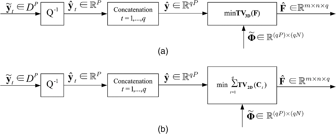
1. Introduction

By the Nyquist–Shannon sampling theory, to reconstruct a signal without error, the sampling rate must be at least twice the highest frequency of the signal. Compressive sampling (CS), also known as compressed sensing, is an emerging line of work that suggests sub-Nyquist sampling of sparse signals of interest.¹^–³ Rather than collecting an entire Nyquist ensemble of signal samples, CS can reconstruct sparse signals from a small number of (random³ or deterministic⁴) linear measurements via convex optimization,⁵ linear regression,⁶^,⁷ or greedy recovery algorithms.⁸

An example of a CS application that has attracted interest is the “single-pixel camera” architecture,⁹ in which a still image can be produced from significantly fewer captured measurements than the number of desired/reconstructed image pixels. A desirable next-step development is compressive video streaming. In the present work, we consider a video transmission system in which the transmitter/encoder performs pure direct compressed sensing acquisition without the benefits of the familiar sophisticated forms of video encoding. This setup is of interest, for example, in problems that involve large wireless multimedia networks of primitive low-complexity, power-limited video sensors. CS is potentially an enabling technology in this context,¹⁰ as video acquisition would require minimal or no computational power at all, yet transmission bandwidth would still be greatly reduced. In such a case, the burden of quality video reconstruction will fall solely on the receiver/decoder side. In comparison, conventional predictive encoding schemes [H.264¹¹ or high efficiency video coding (HEVC)¹²] are known to offer great transmission bandwidth savings for targeted video quality levels, but place strong complexity and power consumption demands on the encoder side.

The transmission bandwidth and the quality of the reconstructed CS video are determined by the number of collected measurements, which based on CS principles should be proportional to the sparsity level of the signal. The challenge of implementing a well-compressed and well-reconstructed CS-based video streaming system rests on developing effective sparse representations and corresponding video recovery algorithms. Several methods for CS video recovery have already been proposed, each relying on a different sparse representation. An intuitive (JPEG-motivated) approach is to independently recover each frame using the two-dimensional discrete cosine transform (2D-DCT)¹³ or a two-dimensional discrete wavelet transform (2D-DWT).¹⁴ As an improvement that enhances sparsity by exploiting correlations among successive frames, several frames can be jointly recovered under a three-dimensional DWT (3D-DWT)¹⁴ or 2D-DWT applied on inter-frame difference data.¹⁵ To enhance sparse representation and exploit motion among successive video frames, a video sequence is divided into key frames and CS frames in Refs. 16 and 17. Whereas each key frame is reconstructed individually using a fixed basis (e.g., 2D-DWT or 2D-DCT), each CS frame is reconstructed conditionally using an adaptively generated basis from adjacent already reconstructed key frames. In Refs. 18–20, each frame of a compressed-sensed video sequence is reconstructed iteratively using adaptively generated Karhunen–Loève transform (KLT) bases from neighboring frames.

Another approach for compressed-sensed signal recovery is total-variation (TV) minimization. TV minimization, also known as TV regularization, has been widely used in the past as an image denoising algorithm.²¹^,²² Based on the principle that signals with excessive, likely spurious detail have excessively high TV (that is, the integral of the absolute gradient of the signal is high), reducing TV of the reconstructed signal while staying consistent with the collected samples removes unwanted detail while preserving important information such as edges. Recently, 2D-TV minimization algorithms were successfully used in CS image recovery.⁵^,²³^–²⁷ In Refs. 28 and 29, a multiframe CS video encoder was proposed with interframe TV minimization decoding. Although promising, such a system requires complex and expensive spatial-temporal light modulators that make the technique difficult to be implemented in practice.

In this present work, we propose a system that consists of a pure framewise CS video encoder in which each video frame is encoded independently using compressive sensing. Such a CS video acquisition system can be directly implemented practically with existing CS imaging technology. At the receiver/decoder, we develop and describe in detail a procedure by which multiple independently encoded video frames are jointly recovered successfully via sliding window–based interframe TV minimization.

The rest of this paper is organized as follows. In Sec. 2, we briefly review TV-based CS signal recovery principles. In Sec. 3, the proposed framewise CS video acquisition system with interframe TV minimization decoding is described in detail. Some experimental results are presented and examined in Sec. 4, and a few conclusions are drawn in Sec. 5.

2. Compressive Sampling with TV Minimization Reconstruction

In this section, we briefly review 2-D and 3-D signal acquisition by CS and recovery using sparse gradient constraints (TV minimization). If the signal of interest is a 2-D image $X \in R^{m \times n}$ and $x = vec (X) \in R^{N}$ , $N = m n$ , represents vectorization of $X$ via column concatenation, then CS measurements of $X$ are collected in the form of

Eq. (1)

y = Φ vec (X),

with a linear measurement matrix

Φ_{P \times N}

,

P ≪ N

. Under the assumption that images are mostly pixelwise smooth in the horizontal and vertical pixel directions, it is natural to consider utilizing the sparsity of the spatial gradient of

X

for CS image reconstruction.⁵^,²³^–²⁷ If

x_{i, j}

denotes the pixel in the

i

’th row and

j

’th column of

X

, the horizontal and vertical gradients at

x_{i, j}

are defined, respectively, as

D_{h; i j} [X] = {\begin{cases} x_{i, j + 1} - x_{i, j}, & j < n, \\ 0, & j = n, \end{cases}

and

D_{v; i j} [X] = {\begin{cases} x_{i + 1, j} - x_{i, j}, & i < m, \\ 0, & i = m . \end{cases}

The discrete spatial gradient of

X

at pixel

x_{i, j}

can be interpreted as the 2D vector

Eq. (2)

D_{i j} [X] = (\begin{matrix} D_{h; i j} [X] \\ D_{v; i j} [X] \end{matrix}),

and the anisotropic 2D-TV of

X

is simply the sum of the magnitudes of this discrete gradient at every pixel,

Eq. (3)

{TV}_{2 D} (X) ≜ \sum_{i j} (| D_{h; i j} [X] | + | D_{v; i j} [X] |) = \sum_{i j} {‖ D_{i j} [X] ‖}_{l_{1}} .

To reconstruct

X

, we can solve the convex program

Eq. (4)

\hat{X} = \underset{\tilde{X}}{argmin} {TV}_{2 D} (\tilde{X}) subject to y = Φ vec (\tilde{X}) .

However, in practical situations the measurement vector

y

may be corrupted by noise. Then, CS acquisition of

X

can be formulated as

Eq. (5)

y = Φ vec (X) + e,

where

e

is the unknown noise vector bounded by a presumably known power amount

‖ e ‖_{l_{2}} \leq ϵ

,

ϵ > 0

. To recover

X

, we can use 2D-TV minimization as in Eq. (4) with a relaxed constraint in the form of

Eq. (6)

\hat{X} = \underset{\tilde{X}}{argmin} {TV}_{2 D} (\tilde{X}) subject to {‖ y - Φ vec (\tilde{X}) ‖}_{l_{2}} \leq ϵ .

Moving on now to the needs of the specific CS video work presented in this paper, if the underlying signal is a video signal $F \in R^{m \times n \times q}$ representing a stack of $q$ successive frames $F_{t} \in R^{m \times n}$ , $t = 1, \dots, q$ , then concatenating the columns of all $F_{1}, \dots, F_{q}$ results to a length $m n q$ vector $f = vec (F)$ . If $f_{i, j, t}$ denotes the pixel at the $i$ th row and $j$ th column of frame $F_{t}$ , then the horizontal, vertical, and temporal gradient at $f_{i, j, t}$ can be defined, respectively, as

D_{h; i j} [F_{t}] = {\begin{cases} f_{i, j + 1, t} - f_{i, j, t}, & j < n, \\ 0, & j = n, \end{cases}

D_{v; i j} [F_{t}] = {\begin{cases} f_{i + 1, j, t} - f_{i, j, t}, & i < m, \\ 0, & i = m, \end{cases}

and

D_{t; i j} [F_{t}] = {\begin{cases} f_{i, j, t + 1} - f_{i, j, t}, & t < q, \\ f_{i, j, 1} - f_{i, j, t}, & t = q . \end{cases}

Correspondingly, the spatial-temporal gradient of

F

at

f_{i, j, t}

can be interpreted as the 3D vector

Eq. (7)

D_{i j} [F_{t}] = (\begin{matrix} D_{h; i j} [F_{t}] \\ D_{v; i j} [F_{t}] \\ D_{t; i j} [F_{t}] \end{matrix}),

and the anisotropic 3D-TV of

F

is simply the sum of the magnitudes of this discrete gradient at every pixel:

Eq. (8)

{TV}_{3 D} (F) ≜ \sum_{i, j, t} (| D_{h; i j} [F_{t}] | + | D_{v; i j} [F_{t}] | + | D_{t; i j} [F_{t}] |) = \sum_{i, j, t} {‖ D_{i j} [F_{t}] ‖}_{l_{1}} .

To reconstruct the frame sequence

F

from noiseless measurements, we can solve the convex program

Eq. (9)

\hat{F} = \underset{\tilde{F}}{argmin} {TV}_{3 D} (\tilde{F}) subject to y = Φ vec (\tilde{F}) .

The reconstruction of

F

from noisy measurements can be formulated as the 3D-TV decoding

Eq. (10)

\hat{F} = \underset{\tilde{F}}{argmin} {TV}_{3 D} (\tilde{F}) subject to {‖ y - Φ vec (\tilde{F}) ‖}_{l_{2}} \leq ϵ .

If the individual frames $F_{1}, \dots, F_{q}$ in $F$ are highly time-correlated, then a pixelwise temporal DCT generally improves sparsity. As illustrated in Fig. 1, each temporal-length $q$ ( $q = 4$ for example) vector $f_{i, j} = {[f_{i, j, 1}, \dots, f_{i, j, q}]}^{T}$ , $i = 1, \dots, m$ , $j = 1, \dots, n$ , consisting of the pixels at spatial position $(i, j)$ across $q$ successive frames, can be represented as

Eq. (11)

f_{i, j} = Ψ_{DCT} c_{i, j},

where

Ψ_{DCT}

is the 1D-DCT basis and

c_{i, j}

is the transform-domain coefficient vector. The resulting coefficient matrix

C_{1}

represents the frequency component that remains unchanged over time (dc) and the subsequent coefficient matrices

C_{t}

,

t = 2, \dots, q

, represent frequency components of increasing time variability. Because each matrix

C_{t}

,

t = 1, \dots, q

, is expected to have small TV, they can be jointly recovered in the form of

Eq. (12)

{\hat{C}}_{1}, \dots, {\hat{C}}_{q} = \underset{{\tilde{C}}_{1}, \dots, {\tilde{C}}_{q}}{argmin} \sum_{t = 1}^{q} {TV}_{2 D} ({\tilde{C}}_{t}) subject to {‖ y - Φ vec ({DCT}^{- 1} ({\tilde{C}}_{1}, \dots, {\tilde{C}}_{q})) ‖}_{l_{2}} \leq ϵ,

where

{DCT}^{- 1} ({\tilde{C}}_{1}, \dots, {\tilde{C}}_{q})

stands for pixelwise inverse 1D-DCT. Subsequently, the complete frame sequence

F

can be reconstructed simply as

Eq. (13)

\hat{F} = {DCT}^{- 1} ({\hat{C}}_{1}, \dots, {\hat{C}}_{q}) .

Below, we will refer to this form of interframe CS reconstruction as TV-DCT decoding.

Fig. 1

Illustration of pixelwise temporal discrete cosine transform (DCT) ( $q = 4$ ).

3. Proposed CS Video System

CS-based signal acquisition with TV-based reconstruction, as described in Sec. 2, can be applied to video coding. In Refs. 28 and 29, the video frame sequence is divided into cubes, and each cube consisting of multiple frames is vectorized and compressed-sensed using a large-scale sensing matrix. At the decoder, each cube of video frames is recovered from the received measurements via 3D-TV decoding as in Eq. (10) or via TV-DCT decoding as in Eqs. (12) and (13). However, such a multiframe CS acquisition system requires simultaneous access—hence, some form of temporal storage—to the whole cube of frames, which is impractical and, arguably, defies the core intention of compressed sensing. In this paper, we propose a practical CS video acquisition system that performs pure, direct framewise encoding. In the simple compressive video encoding block diagram shown in Fig. 2, each frame $F_{t}$ of size $m \times n$ , $t = 1, 2, \dots, T$ , is viewed as a vectorized column $f_{t} \in R^{N}$ , $N = m n$ , $t = 1, 2, \dots, T$ . CS is performed by projecting $f_{t}$ onto a $P \times N$ random measurement matrix $Φ_{t}$ ,

Eq. (14)

y_{t} = Φ_{t} f_{t}, t = 1, 2, \dots, T,

where

Φ_{t}

,

t = 1, 2, \dots, T

, is generated by randomly permuting the columns of an order-

k

,

k \geq N

and multiple-of-four, Walsh–Hadamard (WH) matrix followed by arbitrary selection of

P

rows from the

k

available WH rows (if

k > N

, only

N

arbitrary columns are utilized). This class of WH measurement matrices has the advantage of easy implementation (antipodal

\pm 1

entries), fast transformation, and satisfactory reconstruction performance, as we will see later on. A richer class of matrices can be found in Refs. 30 and 31. To quantize the elements of the resulting measurement vector

y_{t} \in R^{P}

(block

Q

in Fig. 2), in this work we follow a simple adaptive quantization approach of two codeword lengths. A positive threshold

η > 0

is chosen such that 1% of the elements in

y_{1}

have magnitude above

η

. For every measurement vector

y_{t}

,

t = 1, 2, \dots,

16-bit uniform scalar quantization is used for elements with magnitudes larger than

η

, and 8-bit uniform scalar quantization is used for the remaining elements. The resulting quantized values

{\tilde{y}}_{t}

are then indexed and transmitted to the decoder.

Fig. 2

Simple framewise compressed sensing (CS) video encoder system with quantization alphabet $D$ .

To reconstruct the independently encoded CS video frames, a simplistic idea is to recover each frame independently via 2D-TV decoding by Eq. (6). However, such a decoding scheme does not exploit the interframe similarities of a video sequence. We propose, instead, to jointly recover multiple individually encoded CS frames via interframe TV minimization. As shown in Fig. 3, the proposed interframe CS video decoder collects and concatenates a group of $q$ dequantized measurement vectors ${\hat{y}}_{t} \in R^{P}$ , $t = 1, \dots, q$ , to form $\hat{y} \in R^{q P}$ . Because each individual dequantized vector is in the form of ${\hat{y}}_{t} = Φ_{t} f_{t} + e_{t}$ with noise $e_{t}$ , $\hat{y}$ can be represented as

Eq. (15)

\hat{y} = \tilde{Φ} f + e,

where

\tilde{Φ} \in R^{(q P) \times (q N)}

is the block diagonal matrix

Eq. (16)

\tilde{Φ} = (\begin{matrix} Φ_{1} \\ Φ_{2} \\ ⋱ \\ Φ_{q} \end{matrix}),

f

is the concatenation of the

q

vectorized frames

Eq. (17)

f^{T} = [f_{1}^{T} f_{2}^{T} \dots f_{q}^{T}],

and

e

is the concatenation of the noise vectors in the form of

Eq. (18)

e^{T} = [e_{1}^{T} e_{2}^{T} \dots e_{q}^{T}] .

The decoder then performs 3D-TV decoding on the

q

frames [Fig. 3(a)] by

Eq. (19)

\hat{F} = \underset{\tilde{F}}{\arg \min} {TV}_{3 D} (\tilde{F}) subject to {‖ \hat{y} - \tilde{Φ} vec (\tilde{F}) ‖}_{ℓ_{2}} \leq ϵ .

Fig. 3

(a) Proposed 3-D total variation (TV). (b) TV-DCT CS decoder on individually encoded frames.

Although Eq. (19) may be considered a powerful joint 3D-TV recovery procedure for general 2D CS-acquired video, for highly temporally correlated video frames, better reconstruction quality may be achieved via TV-temporal-DCT decoding [Fig. 3(b)] in the form of

Eq. (20)

{\hat{C}}_{1}, \dots, {\hat{C}}_{q} = \underset{{\tilde{C}}_{1}, \dots, {\tilde{C}}_{q}}{\arg \min} \sum_{t = 1}^{q} {TV}_{2 D} ({\tilde{C}}_{t}) subject to {‖ \hat{y} - \tilde{Φ} vec ({DCT}^{- 1} ({\tilde{C}}_{1}, \dots, {\tilde{C}}_{q})) ‖}_{ℓ_{2}} \leq ϵ .

F

can then be reconstructed simply by

Eq. (21)

\hat{F} = {DCT}^{- 1} ({\hat{C}}_{1}, \dots, {\hat{C}}_{q}) .

In Eqs. (20) and (21), we carried out interframe decoding for each independent group of $q$ frames. To further exploit interframe similarities and capture local motion among adjacent groups of frames, we now propose a sliding-window TV-DCT decoder. The concept of such a decoder is depicted in Fig. 4. Initially, the decoder performs TV-DCT decoding on the first $q$ ( $q = 4$ , for example) frames, $F_{1}, \dots, F_{q}$ specified by a decoding window of length $q$ [Fig. 4(a)] using the block diagonal matrix $\tilde{Φ}$ with diagonal elements $Φ_{1}, \dots, Φ_{q}$ . The reconstructed frames are called ${\hat{F}}_{1, 1}$ , ${\hat{F}}_{2, 1}$ , ${\hat{F}}_{3, 1}$ , ${\hat{F}}_{4, 1}$ [Fig. 4(b)], where ${\hat{F}}_{t, l}$ represents the $l$ ’th reconstruction of the $t$ ’th frame. Then, the decoding window shifts one frame to the right, performs TV-DCT decoding on $F_{2}, \dots, F_{q + 1}$ using the matrix $\tilde{Φ}$ with diagonal elements $Φ_{2}, \dots, Φ_{q + 1}$ , and produces the reconstructed frames ${\hat{F}}_{2, 2}$ , ${\hat{F}}_{3, 2}$ , ${\hat{F}}_{4, 2}$ , ${\hat{F}}_{5, 1}$ . The decoder continues on with sliding-window TV-DCT decoding until the last group of frames $F_{T - q + 1}, \dots, F_{T}$ is recovered. Final reconstruction of each frame ${\hat{F}}_{t}$ is executed by taking the average of all different decodings in the form of

Eq. (22)

{\hat{F}}_{t} = {\begin{cases} \frac{1}{t} \sum_{l = 1}^{t} {\hat{F}}_{t, l}, & 1 \leq t \leq q, \\ \frac{1}{q} \sum_{l = 1}^{q} {\hat{F}}_{t, l}, & q \leq t \leq T - q + 1, \\ \frac{1}{T - t + 1} \sum_{l = 1}^{T - t + 1} {\hat{F}}_{t, l}, & T - q + 2 \leq t \leq T . \end{cases}

Compared to the simple (nonsliding-window) TV-DCT decoder of Eqs. (20) and (21), the sliding-window TV-DCT decoder enforces sparsity for any successive

q

frames in the video sequence. Hence, it protects sharp temporal changes for pixels that have fast motion in any

q

-frame-sequence and smooths intensities for static or slow-motion pixels in the same decoding window.

Fig. 4

Proposed sliding-window TV-DCT CS decoder system.

4. Experimental Results

In this section, we study experimentally the performance of the proposed CS video systems by evaluating the peak signal-to-noise ratio (PSNR) (as well as the perceptual quality) of reconstructed video sequences. Two test sequences, Container and Highway, with CIF resolution $352 \times 288$ pixels and frame rate of $30 frames / s$ , are used. Processing is carried out only on the luminance component.

At our trivial, pure CS encoder side, each frame is handled as a vectorized column of length $N = 101376$ multiplied by a $P \times N$ randomized partial WH matrix $Φ_{t}$ . The sensing matrix $Φ_{t}$ is referred to as varying $Φ_{t}$ if it is independently generated to encode each frame and is referred to as fixed $Φ$ if it is generated only once to encode all frames in the video sequence. The elements of the captured $P$ -dimensional measurement vector are quantized and then transmitted to the decoder. In our experiments, $P = 12672$ , 25344, 38016, 50688, 63360 are used to produce the corresponding bit rates of 3071.7, 6143.4, 9215.1, 12287, and 15358 kbps. (Considering the quantization scheme described in Sec. 3 and frame rate 30 fps, the bit rate can be calculated as $(16 \times 0.01 P + 8 \times 0.99 P) \times 30 / 1000 kbps$ .) With an Intel i5-2410M 2.30-GHz processor, the encoding time per frame is well within 0.1 s, whereas the H.264/AVC JM reference software programmed in C++ requires about 1.55 s with low-complexity configurations.¹¹

At the decoder side, we chose the TVAL3 software²⁸^,²⁹ for reconstruction motivated by its low-complexity and satisfactory recovery performance characteristics. In our experimental studies for the slow-motion Container sequence, five CS video systems are examined: (1) baseline fixed $Φ$ acquisition with frame-by-frame 2D-TV decoding [Eq. (6)]; (2) fixed $Φ$ and (3) varying $Φ_{t}$ acquisition with TV-DCT decoding [Eqs. (20) and (21)]; (4) 3D-TV decoding with fixed $Φ$ [Eq. (19)]; and (5) varying $Φ_{t}$ acquisition with sliding-window TV-DCT decoding [Eqs. (20), (21), and (22)]. For the fast-motion Highway sequence, we show results with fixed $Φ$ for CS acquisition and (1) baseline 2D-TV decoding [Eq. (6)]; (2) 3D-TV decoding [Eq. (19)]; (3) plain TV-DCT decoder [Eqs. (20) and (21)]; and (4) sliding-window TV-DCT decoder [Eqs. (20), (21), and (22)]. For all interframe decoders, $q$ (the frame group size and window size, if pertinent) is chosen empirically to the values shown in Tables 1 and 2.

Table 1

Empirical q values for container.

$P / N$	0.125	0.25	0.375	0.5	0.625
Fixed $Φ$ TV-DCT	20	20	20	20	20
Varying $Φ_{t}$ TV-DCT	2	2	20	20	20
Varying $Φ_{t}$ sliding-windowTV-DCT	2	4	20	20	20
Fixed $Φ$ 3D-TV	20	20	20	20	20

Table 2

Empirical q values for highway.

$P / N$	0.125	0.25	0.375	0.5	0.625
Fixed $Φ$ 3D-TV	20	20	20	20	20
Fixed $Φ$ sliding-windowTV-DCT	4	4	4	4	4
Fixed $Φ$ TV-DCT	4	4	4	4	4

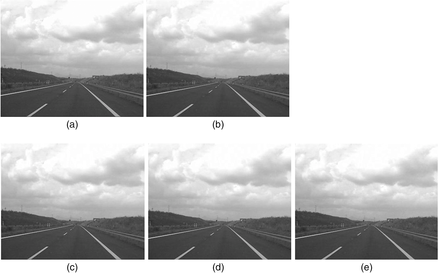
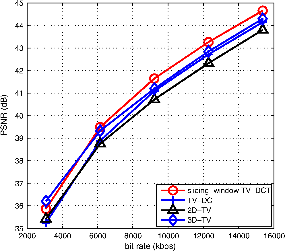
Figure 5 shows the decodings of the 28th frame of Container produced by the sliding-window TV-DCT decoder with varying $Φ_{t}$ and window size $q = 20$ [Fig. 5(b)], the TV-DCT decoder with varying $Φ_{t}$ [Fig. 5(c)], the TV-DCT decoder with fixed $Φ$ [Fig. 5(d)], the 3D-TV decoder with fixed $Φ$ [Fig. 5(e)], and the 2D-TV decoder with fixed $Φ$ [Fig. 5(f)]. It can be observed that the 2D-TV decoder as well as the fixed $Φ$ TV-DCT decoder suffer noticeable performance loss over the whole image, whereas the varying $Φ_{t}$ sliding-window TV-DCT decoder demonstrates considerable reconstruction quality improvement. (As usual, pdf formatting of the present article tends to dampen perceptual quality differences between Fig. 5(a)–5(f) that are quite pronounced in video playback. Figure 6 is the usual attempt to capture average differences quantitatively.) These findings are consistent with the belief that varying $Φ_{t}$ , $t = 1, \dots, q$ , in Eq. (16) results in a joint block-diagonal recovery matrix $\tilde{Φ}$ that is more likely to satisfy the restricted isometry property (RIP)³ for a given data sparsity level.

Fig. 5

Different decodings of the 28th frame of Container ( $P = 0.625 N$ ). (a) Original frame. (b) Sliding-window TV-DCT (varying $Φ_{t}$ , $q = 20$ ). (c) Plain TV-DCT (varying $Φ_{t}$ , $q = 20$ ). (d) Plain TV-DCT (fixed $Φ$ , $q = 20$ ). (e) 3D-TV (fixed $Φ$ , $q = 20$ ). (f) 2D-TV (fixed $Φ$ ).

Fig. 6

Rate–distortion studies on the Container sequence.

Figure 6 shows the rate-distortion characteristics of the five decoders for the Container video sequence. The PSNR values (in dB) are averaged over 100 frames. Evidently, the varying $Φ_{t}$ TV-DCT decoder outperforms the fixed $Φ$ TV-DCT decoder for all $P$ values, as well the fixed $Φ$ 2D-TV decoder at the median–low to high bit rate range with gains as much as 5 dB. The proposed varying $Φ_{t}$ sliding-window TV-DCT decoder further improves performance by up to an additional 2.5 dB.

For the Highway sequence with fixed $Φ$ framewise CS acquisition, Fig. 7 shows the decodings of the 54th frame produced by the sliding-window TV-DCT decoder with window size $q = 4$ [Fig. 7(b)], plain TV-DCT with group size $q = 4$ [Fig. 7(c)], 3D-TV decoder with group size $q = 20$ [Fig. 7(d)], and baseline 2D-TV decoder [Fig. 7(e)]. By Fig. 8, the proposed sliding-window TV-DCT decoder outperforms both the 2D-TV decoder and the 3D-TV decoder at median–low to high bit rate range, as well as the nonsliding-window TV-DCT decoder.

Fig. 7

Different decodings of the 54th frame of Highway ( $P = 0.625 N$ ). (a) Original frame. (b) Sliding-window TV-DCT (fixed $Φ$ , $q = 4$ ). (c) Plain TV-DCT (fixed $Φ$ , $q = 4$ ). (d) 3D-TV (fixed $Φ$ , $q = 20$ ). (e) 2D-TV (fixed $Φ$ ).

Fig. 8

Rate–distortion studies on the Highway sequence.

5. Conclusions

We propose an interframe TV minimizing decoder for video streaming systems with plain framewise CS encoding. Each group of successive frames is jointly decoded by minimizing the TV of the pixelwise DCT along the temporal direction (TV-DCT decoding). To capture local motion across adjacent frames, a sliding-window decoding structure was developed in which a decoding window specifies the group of frames to be decoded. As the window continuously shifts forward one frame at a time, multiple decodings are produced for each frame in the video sequence, from which the average is taken to form the final reconstructed frame. Experimental results demonstrate that the proposed sliding-window interframe TV minimizing decoder outperforms significantly the intraframe 2D-TV minimizing decoder, as well as 3D-TV CS decoding schemes. In terms of future work, to further reduce our encoder/decoder complexity and maintain satisfactory video reconstruction quality, we may develop block-level CS video acquisition systems with rate-adaptive sampling at the encoder and measurement matrices of deterministic design to facilitate efficient encoding/decoding.

Acknowledgments

This work was supported in part by the National Science Foundation (Grant CNS-1117121).

References

1.

E. CandèsT. Tao, “Near optimal signal recovery from random projections: universal encoding strategies?,” IEEE Trans. Inform. Theory, 52 (12), 5406 –5425 (2006). http://dx.doi.org/10.1109/TIT.2006.885507 IETTAW 0018-9448 Google Scholar

2.

D. L. Donoho, “Compressed sensing,” IEEE Trans. Inform. Theory, 52 (4), 1289 –1306 (2006). http://dx.doi.org/10.1109/TIT.2006.871582 IETTAW 0018-9448 Google Scholar

3.

E. CandèsM. B. Wakin, “An introduction to compressive sampling,” IEEE Signal Proc. Mag., 25 (2), 21 –30 (2008). http://dx.doi.org/10.1109/MSP.2007.914731 ISPRE6 1053-5888 Google Scholar

4.

K. Gaoet al., “Compressive sampling with generalized polygons,” IEEE Trans. Signal Proc., 59 (10), 4759 –4766 (2011). http://dx.doi.org/10.1109/TSP.2011.2160860 ITPRED 1053-587X Google Scholar

5.

E. CandèsJ. RombergT. Tao, “Stable signal recovery from incomplete and inaccurate measurements,” Comm. Pure Appl. Math., 59 (8), 1207 –1223 (2006). http://dx.doi.org/10.1002/(ISSN)1097-0312 CPMAMV 0010-3640 Google Scholar

6.

R. Tibshirani, “Regression shrinkage and selection via the lasso,” J. Roy. Stat. Soc. Ser. B, 58 (1), 267 –288 (1996). 1369-7412 Google Scholar

7.

B. Efronet al., “Least angle regression,” Ann. Statist., 32 (2), 407 –451 (2004). http://dx.doi.org/10.1214/009053604000000067 ASTSC7 0090-5364 Google Scholar

8.

J. TroppA. Gilbert, “Signal recovery from random measurements via orthogonal matching pursuit,” IEEE Trans. Inform. Theory, 53 (12), 4655 –4666 (2007). http://dx.doi.org/10.1109/TIT.2007.909108 IETTAW 0018-9448 Google Scholar

9.

M. F. Duarteet al., “Single-pixel imaging via compressive sampling,” IEEE Signal Proc. Mag., 25 (2), 83 –91 (2008). http://dx.doi.org/10.1109/MSP.2007.914730 ISPRE6 1053-5888 Google Scholar

10.

S. PudlewskiT. MelodiaA. Prasanna, “Compressed-sensing-enabled video streaming for wireless multimedia sensor networks,” IEEE Trans. Mobile Comp., 11 (6), 1060 –1072 (2012). http://dx.doi.org/10.1109/TMC.2011.175 ITMCCJ 1536-1233 Google Scholar

11.

I. E. Richardson, The H.264 Advanced Video Compression Standard, 2nd ed.Wiley, New York (2010). Google Scholar

12.

G. J. Sullivanet al., “Overview of the high efficiency video coding (HEVC) standard,” IEEE Trans. Circ. Syst. Video Technol., 22 (12), 1649 –1668 (2012). http://dx.doi.org/10.1109/TCSVT.2012.2221191 ITCTEM 1051-8215 Google Scholar

13.

V. StankovicL. StankovicS. Cheng, “Compressive video sampling,” in Proc. European Signal Proc. Conf. (EUSIPCO), (2008). Google Scholar

14.

M. B. Wakinet al., “Compressive imaging for video representation and coding,” in Proc. Picture Coding Symposium (PCS), (2006). Google Scholar

15.

R. F. MarciaR. M. Willet, “Compressive coded aperture video reconstruction,” in Proc. European Signal Proc. Conf. (EUSIPCO), (2008). Google Scholar

16.

H. W. ChenL. W. KangC. S. Lu, “Dynamic measurement rate allocation for distributed compressive video sensing,” in Proc. Visual Comm. and Image Proc. (VCIP), (2010). Google Scholar

17.

J. Y. ParkM. B. Wakin, “A multiscale framework for compressive sensing of video,” in Proc. Picture Coding Symposium (PCS), (2009). Google Scholar

18.

Y. Liuet al., “Motion compensation as sparsity-aware decoding in compressive video streaming,” in Proc. 17th Intern. Conf. on Digital Signal Processing (DSP 2011), 1 –5 (2011). Google Scholar

19.

Y. LiuM. LiD. A. Pados, “Decoding of purely compressed-sensed video,” Proc. SPIE, 8365 83650L (2012). http://dx.doi.org/10.1117/12.920320 Google Scholar

20.

Y. LiuM. LiD. A. Pados, “Motion-aware decoding of compressed-sensed video,” IEEE Trans. Circ. Syst. Video Technol., 23 (3), 438 –444 (2013). http://dx.doi.org/10.1109/TCSVT.2012.2207269 ITCTEM 1051-8215 Google Scholar

21.

L. RudinS. OsherE. Fatemi, “Nonlinear total variation based noise removal algorithms,” Physica D, 60 (1–4), 259 –268 (1992). http://dx.doi.org/10.1016/0167-2789(92)90242-F PDNPDT 0167-2789 Google Scholar

22.

J. YangY. ZhangW. Yin, “An efficient TVL1 algorithm for deblurring of multichannel images corrupted by impulsive noise,” SIAM J. Sci. Comput., 31 (4), 2842 –2865 (2009). http://dx.doi.org/10.1137/080732894 SJOCE3 1064-8275 Google Scholar

23.

E. CandèsJ. Romberg, “

ℓ

1-magic: recovery of sparse signals via convex programming,” (2005) http://users.ece.gatech.edu/justin/l1magic/downloads/l1magic.pdf Google Scholar

24.

M. LustigD. DonohoJ. M. Pauly, “Sparse MRI: the application of compressed sensing for rapid MR imaging,” Magn. Reson. Med., 58 (6), 1182 –1195 (2007). http://dx.doi.org/10.1002/(ISSN)1522-2594 MRMEEN 0740-3194 Google Scholar

25.

S. Maet al., “An efficient algorithm for compressed MR imaging using total variation and wavelets,” in Proc. IEEE Conf. Comp. Vis. Pattern Recogn., 1 –8 (2008). Google Scholar

26.

C. Li, “An efficient algorithm for total variation regularization with applications to the single pixel camera and compressive sensing,” Rice University, Houston, TX, (2009). Google Scholar

27.

M. R. DadkhahS. ShiraniM. J. Deen, “Compressive sensing with modified total variation minimization algorithm,” in Proc. IEEE Intern. Conf. Acoustics Speech Signal Proc. (ICASSP), 1310 –1313 (2010). Google Scholar

28.

C. Liet al., “Video coding using compressive sensing for wireless communications,” in Proc. IEEE Wireless Commun. Networking Conf. (WCNC), 2077 –2082 (2011). Google Scholar

29.

H. Jianget al., “Scalable video coding using compressive sensing,” Bell Labs Techn. J., 16 (4), 149 –169 (2012). http://dx.doi.org/10.1002/bltj.20539 1089-7089 Google Scholar

30.

H. GanapathyD. A. PadosG. N. Karistinos, “New bounds and optimal binary signature sets—part I: periodic total squared correlation,” IEEE Trans. Commun., 59 (4), 1123 –1132 (2011). http://dx.doi.org/10.1109/TCOMM.2011.020411.090404 IECMBT 0090-6778 Google Scholar

31.

H. GanapathyD. A. PadosG. N. Karistinos, “New bounds and optimal binary signature sets - part II: aperiodic total squared correlation,” IEEE Trans. Commun., 59 (5), 1411 –1420 (2011). http://dx.doi.org/10.1109/TCOMM.2011.020811.090405 IECMBT 0090-6778 Google Scholar

Biography

Ying Liu received the BS degree in telecommunications engineering from Beijing University of Posts and Telecommunications, Beijing, China, in 2006, and the PhD degree in electrical engineering from the State University of New York at Buffalo, Buffalo, New York, in 2012. Her research interests include video streaming, compressed sensing, and adaptive signal processing. She is currently an air traffic control engineer with ARCON Corp., Waltham, Massachusetts.

Dimitris A. Pados received the diploma degree in computer science and engineering from the University of Patras, Greece, in 1989, and the PhD degree in electrical engineering from the University of Virginia, Charlottesville, Virginia, in 1994. From 1994 to 1997, he held an assistant professor position in the Department of Electrical and Computer Engineering and the Center for Telecommunications Studies, University of Louisiana, Lafayette. Since August 1997, he has been with the Department of Electrical Engineering, State University of New York at Buffalo, where he is presently a professor. His research interests are in the general areas of communication theory and adaptive signal processing. He received a 2001 IEEE International Conference on Telecommunications best paper award, the 2003 IEEE Transactions on Neural Networks Outstanding Paper Award, and the 2010 IEEE International Communications Conference Best Paper award in Signal Processing for Communications for articles that he coauthored with students and colleagues. He is a recipient of the 2009 SUNY system-wide Chancellor’s Award for Excellence in Teaching and the 2011 University at Buffalo Exceptional Scholar—Sustained Achievement Award.

CC BY: © The Authors. Published by SPIE under a Creative Commons Attribution 4.0 Unported License. Distribution or reproduction of this work in whole or in part requires full attribution of the original publication, including its DOI.

Citation Download Citation

Ying Lu and Dimitris A. Pados "Decoding of framewise compressed-sensed video via interframe total variation minimization," Journal of Electronic Imaging 22(2), 021012 (8 April 2013). https://doi.org/10.1117/1.JEI.22.2.021012

Published: 8 April 2013

Access the abstract

JOURNAL ARTICLE
9 PAGES

DOWNLOAD PAPER SAVE TO MY LIBRARY

GET CITATION

CITATIONS

Cited by 12 scholarly publications.

Explore citations on Lens.org

KEYWORDS

Video

Video compression

Compressed sensing

Video coding

Computer programming

Reconstruction algorithms

Quantization

Show All Keywords

CHORUS Article. This article was made freely available starting 08 April 2014

1.

Introduction

2.

Compressive Sampling with TV Minimization Reconstruction

Eq. (1)

Eq. (2)

Eq. (3)

Eq. (4)

Eq. (5)

Eq. (6)

Eq. (7)

Eq. (8)

Eq. (9)

Eq. (10)

Eq. (11)

Eq. (12)

Eq. (13)

Fig. 1

3.

Proposed CS Video System

Eq. (14)

Fig. 2

Eq. (15)

Eq. (16)

Eq. (17)

Eq. (18)

Eq. (19)

Fig. 3

Eq. (20)

Eq. (21)

Eq. (22)

Fig. 4

4.

Experimental Results

Table 1

Table 2

Fig. 5

Fig. 6

Fig. 7

Fig. 8

5.

Conclusions

Acknowledgments

References

Biography

Show All Keywords

Keywords/Phrases

Search In:

Publication Years