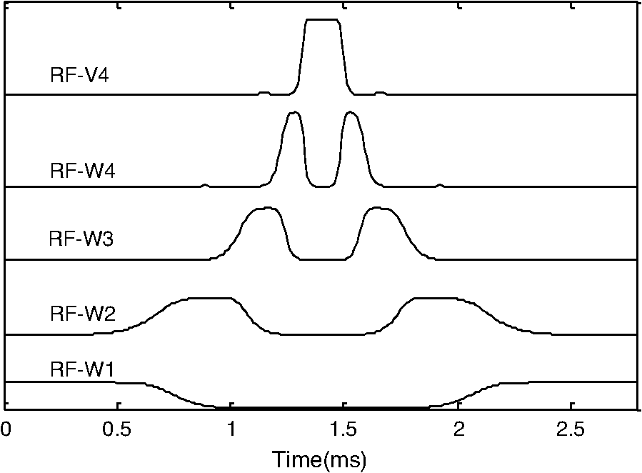
1.

Introduction

In conventional magnetic resonance imaging (MRI), scanners acquire samples of the encoded image in a spatial frequency (Fourier) domain, which is called $k$-space. The MR image of the object in the spatial domain can be reconstructed through inverse Fourier transform of the $k$-space data.¹ A well-known problem in MRI is its long scan time that depends on the required number of acquired samples determined through Shannon-Nyquist sampling theory. Potential reconstruction of MR images from a reduced number of acquired samples without degrading the image quality would offer an effective method to reduce scan time while improving the resolution of current MR imagers. However, insufficient sampling of $k$-space data violates the Shannon-Nyquist criterion and produces aliasing artifacts and noise in reconstructed MR images. Several common approaches to alleviate these artifacts and noise are to exploit redundancies in $k$-space and to use temporal filtering, such as partial-Fourier, variable-density sampling, unaliasing by Fourier-encoding the overlaps using the temporal dimension (UNFOLD), etc.^2–5 However, these methods still do not overcome low sampling rate artifacts. Investigations on the feasibility of wavelet encoding in MRI demonstrated better flexibility and adaptability in MR data acquisition than Fourier encoding.^6–8 Unfortunately, the practicality of wavelet encoding in faster acquisition of MRI data has not been demonstrated in the above efforts.

Through recent developments in the theory of compressive sensing (CS), MR images with a sparse representation in some transform domain, under the constraint of incoherent measurement, can be recovered from “randomly” under sampled $k$-space.^9,10 CS theory here exploits such sparsity of MRI data and reconstructs an MR image from very few incoherent measurements through a nonlinear procedure. Several methods have applied CS to Fourier-encoded MRI to reduce scan time.^10–17 These methods are based on two characteristics of conventional MRI: MR images are naturally compressible in certain transform domains, and the sampling pattern is incoherent with respect to some sparsifying transformations. The natural fit of CS to MRI is discussed¹⁰ by reviewing the constraints required for successful reconstruction. Lustig et al.¹¹ have applied CS to recover MR images from a subset of Fourier-encoded $k$-space acquired by pseudo-random variable-density under sampling of phase-encoding to achieve fast imaging. The discrete cosine transforms (DCT), wavelet transform and finite-difference transform were used to exploit the sparsity of brain and angiogram MR images. The incoherence between these sparsifying transforms and Fourier operator were measured by the point spread function (PSF), and transform PSF (TPSF), whereas variable density random under sampling was used to improve the degree of incoherence. As their results showed, this CS approach achieved high reduction of imaging time in three-dimensional (3-D) Fourier-encoded imaging with good reconstruction performance. However, in two-dimensional (2-D) Fourier-encoded MRI, this approach does not achieve such benefit because only one-dimensioanl (1-D) sparsity was exploited.

In mathematical CS theory, Fourier basis is maximally incoherent with the canonical basis.^9,18 In traditional MRI, because the $k$-space data are encoded by Fourier basis, the incoherent measurement constraint is only satisfied when the MR signal is sparse in the spatial domain. Consequently, it can be seen¹¹ that CS-MRI is more suitable for angiogram imaging than for brain imaging because angiograms are sparse in their pixel representation. Therefore, Fourier-encoded MRI is not a good encoding scheme for stable and accurate CS reconstruction in most scenarios where MR signals are not sparse in the spatial domain. In addition, some existing crucial limitations remain unresolved in Fourier-encoded MRI, such as optimization of sampling trajectories and the computation time of reconstruction algorithms.

Several studies have also investigated non-Fourier MRI and CS schemes to reduce the image acquisition time while improving the reconstruction quality.^19–21 Random encoding of $k$-space is achieved by tailoring spatially selective RF pulses to satisfy CS constraints in non-Fourier domains,¹⁹ achieving impressive reconstruction results. The CS constraints are satisfied better by making the energy of $k$-space spread out in non-Fourier domain and pseudo 2-D random sampling.^20,21 Despite the potential of the CS approaches in non-Fourier MRI to outperform traditional Fourier MRI, no general CS approach has yet been developed with strict theoretical justification.

Recent research on application of CS to fast MRI suggests that there is no theoretical performance guarantee for CS-MRI with or without random encoding, and new CS based methods should be developed for specific applications.¹⁹

In recently published CS papers, adaptive sampling in the wavelet domain has been proposed to improve the signal recovery performance.^22,23 Adaptive sampling schemes exploiting the tree structure of nonzero wavelet signal coefficients have been used to replace the ‘universal’ acquisition of random or pseudo-random sampling in traditional CS methodology.^22,23 These schemes use nonrandom sampling and allow more control over the sensing procedure in the form of feedback to improve the CS performance significantly with fewer measurements and higher reconstruction quality. Haupt et al., have demonstrated that the adaptive sampling in CS, called compressive distilled sensing, has the advantage of significantly improving the error bounds compared to traditional CS schemes without adaptive sampling.²⁴ These adaptive strategies have the potential to achieve more accurate and robust signal recovery in some practical applications.²⁵ Therefore, if adaptive sampling is used in wavelet-encoded CS-MRI, it is possible to improve the reconstruction quality of images. We introduced well-known adaptive sampling in the wavelet domain, as used in image compression,^26–28 to encode the MRI data yielding good reconstruction quality.

In this paper, an efficient implementation of a specific CS approach in a simulator that allows good MRI reconstruction from a sparse wavelet-encoded $k$-space following the well-known embedded zero-tree structure for image coding is presented.^26–28 With this approach, sparsity of image data in the spatial domain is not required. In wavelet-encoded MRI, the $k$-space data are encoded in multiple levels in the wavelet domain.⁶ The multilevel decomposed image is then transformed into a vector of sparse wavelet coefficients, and these few significant coefficients are encoded to reconstruct the image with high fidelity.²⁶ Therefore, it is possible to represent the $k$-space data with only a few significant samples and still reconstruct an MR image with a reduced scan time. Additionally, the reconstruction quality of such under sampled $k$-space may be guaranteed by using the input vector of sparse wavelet coefficients in a specific CS framework. The following sections will discuss the proposed CS-MRI approach in the wavelet domain to achieve fast imaging and assess the reconstruction performance at different sampling rates, noise and sparsity levels. Section 2 introduces the procedure of sparse acquisition in wavelet-encoded MRI through the description of RF pulse definition, pulse sequence implementation and adaptive $k$-space trajectories in a simulator. Section 3 presents an efficient CS algorithm based on the minimization of total-variation regularization and a least squares measurement of signal to reconstruct MR image from these sparsely encoded $k$-space samples in the wavelet domain. Section 4 discusses the simulation results and reconstruction performance for phantom and brain images. Section 5 describes feasibility of future applications of our work.

2.

Implementation of Sparse Data Acquisition in Wavelet-Encoded k-Space

2.3.

Simulation of Sparse MR Data Acquisition in the Wavelet Domain

Most MRI simulators are developed based on the solutions of the Bloch equation, and the generated MR signal is encoded in Fourier domain.^30,31 Wavelet domain simulators were developed in earlier years but did not demonstrate any advantage in MRI scanning time.^6–8 In this paper, a simulator generating MR signal in wavelet domain using adaptive sampling in a CS framework has been developed by designing RF excitation pulses and pulse sequences as described in detail in the following sections. This simulator generating MR signals in the wavelet domain is developed for sparse data acquisition as shown in Fig. 1. The executable code in MATLAB for our simulator can be accessed from the following link: http://www2.ece.ttu.edu/CVIAL/simulators/WaveletCSMRISim.exe. Our simulator is a modified version of a Fourier domain MRI simulator developed by Yoder et al. in 2004.³⁰

Fig. 1

An overview of wavelet-encoded MRI simulator for sparse data acquisition.

2.3.1.

Simulator overview

An overview of the proposed MRI simulator to acquire sparse wavelet-encoded $k$-space data is shown in Fig. 1. In the proposed data acquisition scheme, we do not need the information from fully sampled data. We actually acquire the wavelet-encoded MRI data starting with the lowest resolution $k$-space $W_{-J}$ by designing spatially localized wavelet shaped RF excitation pulses for generating $k$-space trajectory by replacing the traditional phase encoding trajectory. Only the lowest resolution trajectory is fully sampled (requiring a small number of RF excitation pulses and the least data acquisition time) to identify for the significant parent wavelet coefficients and to allow full sampling across the levels if desired. The subsequent finer scale $k$-space {$W_{-j}$, $j=1,2,\dots ,J-1$} data are generated by a multiple (e.g., two to eight for four level wavelet encoding based on the parent–child tree structure of wavelet coefficients) of RF excitation pulses as shown in the encoding overview in Fig. 1 (see Sec. 4.2 for details of implementation). Using a virtual object, scanning parameters, such as $B_0$, $G_x$, $G_y$ (magnetic gradient along $x$ and $y$ axis), flip angle, TE (time echo), TR (time repetition), are initialized first. This simulator generates $k$-space data in multiple levels. For $J$-level imaging, the level $j$ of $k$-space acquisition starts from $J$ to 1. When $j$ equals to $J$, two RF excitation pulses, which are designed, respectively by the $J$’th-level scaling and wavelet functions, are used to generate spin echo signals. After wavelet-encoding and frequency-encoding, the subspaces $V_{-J}$ and $W_{-J}$ are acquired, and then significant samples are tested in $W_{-J}$ to construct {$\mathrm{supp}({\overline{\mathbf{D}}}_{-j})$, $j=1,2,\dots ,J-1$}. When level $j$ is from $J-1$ to 1, RF excitation pulses are designed by $j$’th-level wavelet function and indexed by supp (${\overline{\mathbf{D}}}_{-j}$) to acquire under sampled $k$-space W_-j. Finally, the sparse-encoded $k$-space $\mathit{S}$ is constructed by these subspaces $V_{-J}$, and $W_{-J}$ to $W_{-1}$ to contain all significant samples. To simulate realistic images, noise is added to the $k$-space.

2.3.2.

Design of RF excitation pulses

Excitation profiles in this wavelet-encoded MRI simulator are varied and shaped by functions of wavelet transform. At small flip angles (less than 30 deg), RF pulses are shaped by Fourier transform of excitation profiles. Here, we utilize the Battle-Lemarie wavelet basis functions as shown in Fig. 2 to design RF pulses. Figure 2(a) shows the wavelet scaling and basic functions ${\phi }_{0,0}(x)$ and ${\psi }_{0,0}(x)$ in the spatial domain. The major reason to choose this specific basis function set is that their Fourier transforms are smooth and rapidly decay to zero as shown in Fig. 2(b). This basis set provides short RF pulses with relatively precise spatial excitation profiles.⁶

Fig. 2

Battle-Lemarie functions. (a) Scaling and wavelet basis functions in time domain; (b) Fourier transforms of scaling and wavelet functions.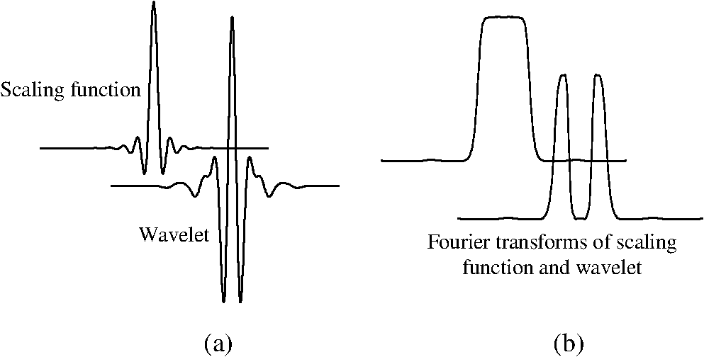

For $J$-level wavelet encoding, assume that the gradient strength along $x$-axis is $G_x$, the FOV along $x$-axis is $X$ centimeters, and the highest resolution is $N$. According to Eqs. (1)-(3), we combine one set of scaling functions {${\phi }_{-J,k}(x)$, $k=0,1,\dots ,N{2}^{-J}-1$} and $J$ sets of wavelets {${\psi }_{-j,k}(x)$, $j=1,\dots J$; $k=0,1,\dots ,N{2}^{-J}-1$} required to shape the excitation profiles. Therefore, ($J+1$) RF pulse profiles ${\mathrm{\Phi }}_{-J,k}$ and {${\mathrm{\Psi }}_{-j,k}$, $j=1,\dots ,J$} are required to generate $k$-spaces $V_{-J}$ and {$W_{-j}$, $j=1,\dots J$}, where ${\mathrm{\Phi }}_{-J,k}$ and {${\mathrm{\Psi }}_{-j,k}$, $j=1,\dots ,J$} are Fourier transforms of ${\phi }_{-J,k}(x)$ and {${\psi }_{-j,k}(x)$, $j=1,\dots ,J$}, respectively. The excited location along $x$-axis is determined by the center carrier frequency of the RF pulse. In order to cover the entire FOV, the fundamental size $\mathrm{\Delta }x$ of translation step is $X/N$. According to the Bloch equation, there is a linear mapping of the resonant frequency ${\omega }_x$ of the spins and the spatial location $x$, i.e., ${\omega }_x=\gamma G_{x}x$, and the fundamental frequency step $\mathrm{\Delta }{\omega }_x=\gamma G_x\mathrm{\Delta }x$, where $\gamma$ is gyromagnetic ratio (approximately $42.58\mathrm{MHz}/\mathrm{T}$ for hydrogen). For small-flip-angle excitation, the carrier frequencies of each pulse in {${\mathrm{\Phi }}_{-J,k}$} and {${\mathrm{\Psi }}_{-j,k}$} are offset by {$k·2^J\mathrm{\Delta }{\omega }_x$} and {$k·2^j\mathrm{\Delta }{\omega }_x$} correspondingly to excite each of the locations {$k·2^J{\mathrm{\Delta }}_x$} and {$k·2^j{\mathrm{\Delta }}_x$}. The duration time $\mathrm{\Delta }t$ of pulse {${\mathrm{\Phi }}_{-J,k}$} is computed by $\mathrm{\Delta }t=1/(2^J\mathrm{\Delta }{\omega }_x)$ and used to compute the half-power width of {${\mathrm{\Phi }}_{-J,k}$}. For example, in 4-level wavelet encoding (e.g., $J=4$), $Gx=1\mathrm{G}/\mathrm{cm}$, $X=25.6\mathrm{cm}$, and $N=256$. Five types of pulse profiles, labeled RF-V4, RF-W4, RF-W3, RF-W2 and RF-W1, are required to produce these RF pulses ${\mathrm{\Phi }}_{-4,k}$ and {${\mathrm{\Psi }}_{-j,k}$, $j=1,\dots ,4$}. The fundamental frequency step $\mathrm{\Delta }{\omega }_x$ is 426 Hz, and the duration time $\mathrm{\Delta }t$ of pulse RF-V4 is approximately 0.15 ms, as shown in Fig. 3. After reconstruction of MR images in the spatial domain, the imaging resolution of 1 mm can be achieved.

Fig. 3

RF pulse profiles for 4-level wavelet encoding.

Any deviation of $G_x$ (e.g., $B_1$ inhomogeneity along $x$-axis) would result in a distortion of excitation profiles, especially occurring in high static field ($B_0\ge 3T$) and with tailored RF pulses. In practice, this distortion can be corrected using a prescan with the same sequence. A fully sampled image acquired for each spatially selective pulse is used as a standard to compute compensation parameters for each excitation profiles.¹⁹ The inhomogeneity maps generated from 3-D images are acquired by prescans and the carrier frequency and amplitude of pulses are adjusted to excite a uniform slice.³² In this paper, if the inhomogeneity maps (e.g., $G_x^{\prime }$) is acquired using prescans, the distortion of excitation profiles can be calibrated by adjusting the carrier frequency of each pulses. In the simplified version of this simulator, we neglect the inhomogeneity in $G_x$ and there is no distortion of excitation profiles.

2.3.3.

Pulse sequences

During MR imaging, the timing of pulse sequences determines the RF signal acquisition and $k$-space trajectories. Pulse sequences contain RF pulses and magnetic field gradients. In wavelet-encoded MRI simulator, the timing of pulse sequences is defined with spatially selective RF excitation and adaptive $k$-space trajectories to yield a sparse encoding scheme.

As shown in Fig. 1, at the beginning, RF pulses {${\mathrm{\Phi }}_{-J,k}$, $k=1,2,\dots ,N·2^{-J}$} and {${\mathrm{\Psi }}_{-J,k}$, $k=1,2,\dots ,N·2^{-J}$} with the carrier frequency offset by {$k·2^J\mathrm{\Delta }{\omega }_x$} are used to generate $J$-level wavelet-shaped excitation profiles along $x$ axis. In the following step, a precession with application of magnetic gradient along $y$ axis is specified by its duration and the gradient magnitude to fill the $k$’th line of frequency-encoding in $k$-space. After $N·2^{-J}$ RF pulses and lines of frequency-encoding, the $k$-space $V_{-J}$ and $W_{-J}$ are fully sampled. In $W_{-J}$, the positions of significant samples, $\mathrm{supp}({\overline{\mathbf{D}}}_{-J})$, are tested by Eq. (4) and then {$\mathrm{supp}({\overline{\mathbf{D}}}_{-j})$, $j=1,2,\dots ,J-1$} are constructed. When $j$ is from $J-1$ to 1, RF pulses {${\mathrm{\Psi }}_{-j,k}$, $k\in \mathrm{supp}({\overline{\mathbf{D}}}_{-j})$} with the carrier frequency offset by {$k·2^j\mathrm{\Delta }{\omega }_x$} and magnetic gradient are applied to achieve the trajectory consisting only of significant samples in $W_{-j}$. Finally, the sparsely encoded $k$-space $\mathit{S}$ constructed by these subspaces $V_{-J}$, $W_{-J}$ to $W_{-1}$ contains the significant samples.

2.3.4.

Noise

In real MRI scanners, the acquired raw $k$-space data are considered to be corrupted by complex white Gaussian noise with the same variance in the real and imaginary parts. After reconstruction of MR images from the corrupted $k$-space data, the noise embedded in the image intensity has Rayleigh statistics in the background and Rician statistics in the signal regions.^33,34 Therefore, this noise model is used in this simulator with different signal to noise ratio (SNR), with SNR is defined as

Eq. (5)

$$\mathrm{SNR}=20{\log }_{10}\frac{A_{\text{signal}}}{A_{\text{noise}}},$$

where $A_{\text{signal}}$ is the average root mean square (RMS) amplitude of the signal, and $A_{\text{noise}}$ is the average RMS amplitude of the noise.

3.

CS Reconstruction of MR images

3.3.

CS Reconstruction Experiment

The numerical experiments for CS reconstruction of 1D piecewise smooth signal {$x[n]$, $n=1,2,\dots ,256$} are performed by 4-level sparse wavelet encoding. The proposed CS reconstruction result from significant wavelet coefficients only, denoted as $x^{*}$, is compared with the best sparse approximation result, denoted as $x^{\prime }$, which includes the zero-filled insignificant coefficients as well.

Figure 4 shows the reconstruction results $x^{*}$ and $x^{\prime }$ with different measurement number $M=60$, 88, 116 and 144. The measurement $\mathit{y}$ at each sampling number is acquired by sparse encoding in the wavelet domain. CS reconstruction performs better than the best sparse approximation reconstruction does with $x^{*}$ approaching the original signal $x$ closely under all conditions. Table 1 shows RIP constants and reconstruction SNRs at different measurement number $M$. Larger values of $M$ result in smaller values of ${\delta }_k$ and higher reconstruction SNRs by CS with better sparse approximation results.

Fig. 4

The reconstruction results with (a) $M=60$, (b) $M=88$, (c) $M=116$ and (d) $M=144$.

Table 1

The RIP constants and SNRs for each sampling number.

$M$	46	60	74	88	102	116	130	144
${\delta }_k$	0.0248	0.0175	0.0119	0.0056	0.0048	0.0008	0.0006	0.0005
SNR(dB) in $x^{*}$	28.80	30.13	30.73	37.47	39.35	42.45	44.09	44.21
SNR(dB) in $x^{\prime }$	12.95	14.55	16.30	17.79	20.16	27.78	28.99	29.88

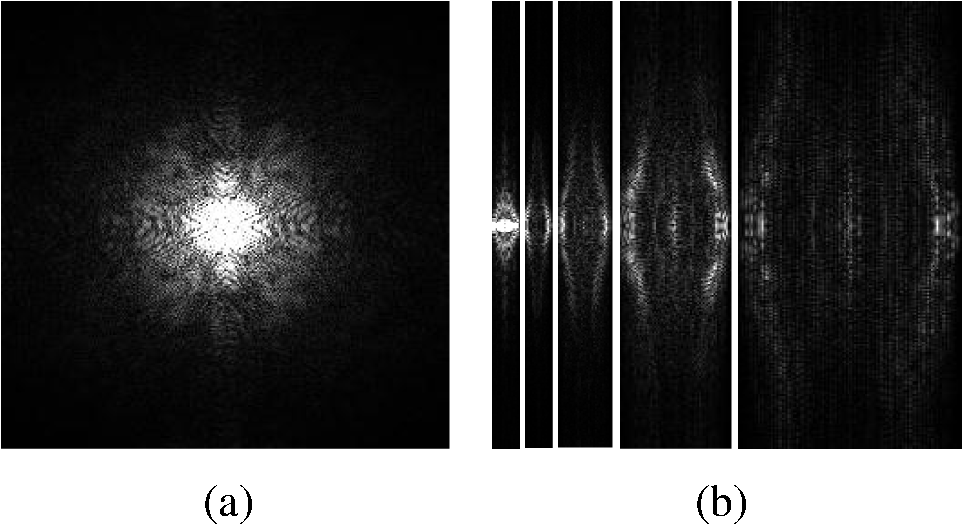
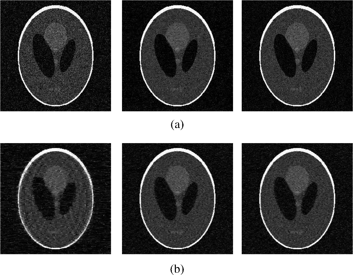
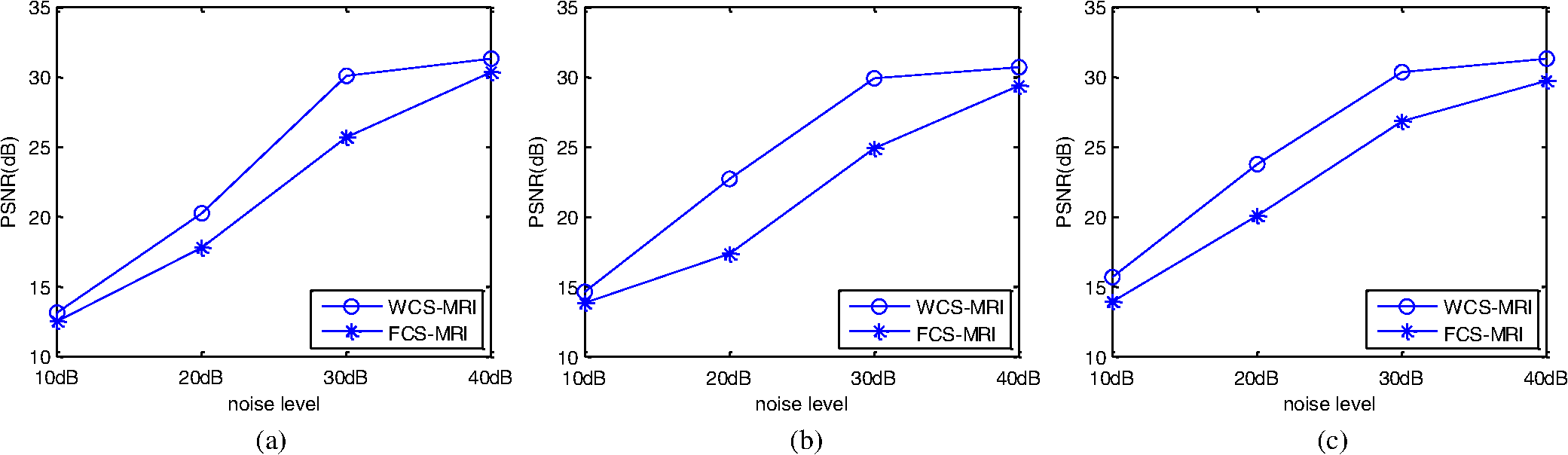
4.

Experimental Results

The Shepp-Logan phantom and a 3-D digital brain phantom from the McConnell Brain Imaging Center, Montreal Neurological Institute, McGill University are used as virtual objects in the MRI simulator to investigate the properties of the proposed wavelet-encoded CS-MRI scheme (WCS-MRI).^41,42 The digital brain phantom has a spatial resolution of $1{\mathrm{mm}}^3$ and contains most of the relevant tissue types. Based on these phantoms, we first simulate the fully sampled wavelet-encoded MRI, and then we simulate the sparse acquisition of $k$-space data at different sampling rates and reconstruct MR images by CS. These simulation results are compared with the results of the commonly used Fourier-encoded CS-MRI scheme (FCS-MRI). In Fourier-encoded $k$-space, most of the energy is concentrated close to the center and rapidly decays toward the periphery. Therefore, a variable-density sampling scheme is implemented in FCS-MRI, where the phase encoding locations are randomly spaced but cover the low-frequency portion near the center of $k$-pace, matching the energy distribution in $k$-space. The CS reconstruction of MR image is performed from the undersampled $k$-space data.

4.1.

Implementation of Wavelet-Encoded MRI Simulation

Data are collected for MR image reconstruction on a $256\times 256$ voxel grid using the Shepp-Logan phantom and two different brain slices (slice 1 and slice 2) from the brain phantom. Figures 5 and 6 show fully sampled Fourier-encoded and 4-level wavelet-encoded MRI results, respectively. These results are generated with zero noise and homogeneous magnetic field ($B_0=3T$). The imaging parameters are $\mathrm{TE}/\mathrm{TR}=25/500\mathrm{ms}$, $\text{read out time}=10\mathrm{ms}$ and $\text{flip angle}=30\mathrm{deg}$. For each image, there are 256 RF excitation pulses required, and its spatial resolution is $256\times 256$. It is seen visually that wavelet-encoded MRI acquires images with the same quality and resolution as Fourier-encoded MRI does. The quantitative assessment of the quality of the reconstructed images has been computed by peak signal to noise ratio (PSNR) and structural similarity (SSIM) as shown in Sec. 4.2.

Fig. 5

Fully sampled Fourier-encoded MR images of (a) the Shepp-Logan phantom, (b) brain image 1 and (c) brain image 2.

Fig. 6

Fully sampled 4-level wavelet-encoded MR images of (a) the Shepp-Logan phantom, (b) brain image 1 and (c) brain image 2.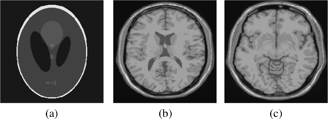

Figure 7 shows the energy of $k$-spaces acquired by Fourier- and wavelet-encoded MRI for brain image 1, respectively. In Fig. 7(a), most of the energy in Fourier-encoded $k$-space is concentrated close to the center of $k$-space, at low spatial frequencies. However, in Fig. 7(b), the wavelet-encoded $k$-space is represented in multiple levels with a high degree predictability between levels. The coarse scale subspace $V_{-4}$ has its spectrum localized in the low frequency band, while these fine scale subspaces $W_{-1}$ to $W_{-4}$ have their energy widely dispersed in the high frequency band and well-organized in trees along wavelet encoding direction.

Fig. 7

Comparison of Fourier and wavelet-encoded $k$-spaces for brain image 1. (a) Fourier-encoded $k$-space; (b) wavelet-encoded $k$-spaces ($L$ to $R$), $V_{-4}$, $W_{-4}$, $W_{-3}$, $W_{-2}$, and $W_{-1}$.

4.2.

Simulation of CS-MRI

The proposed WCS-MRI scheme has been simulated with the phantoms shown in Fig. 5 with different sampling rates. The implementations of sampling patterns reported^22–24 are not the same as our approach. Our data acquisition time is reduced by sparse acquisition of only significant samples across multiple levels by designing appropriate RF excitation pulses at each level. Such wavelet-encoded MRI provides the flexibility and adaptivity to represent the $k$-space data, especially in multiple levels. According to the wavelet decomposition theory, it is possible to achieve the sparse acquisition of $k$-space data by exploiting the hierarchical binary tree structure in the wavelet coefficients set.^6–8,28 Our implementation is based on the structural characteristics of wavelet coefficients and uses a desired percentage of the full samples in our proposed CS-MRI making the acquisition time directly proportional to the sampling rate. Our data acquisition time is reduced by sparse acquisition of only significant samples across multiple levels by designing appropriate RF excitation pulses at each level. For 4-level wavelet-encoded MRI, there are 16 RF excitation pulses required to generate $W_{-4}$ and $V_{-4}$, respectively. If significant samples in $W_{-4}$ are generated by only $m$ RF pulses ($m\le 16$), the corresponding number of RF pulses in $W_{-3}$, $W_{-2}$ and $W_{-1}$ are $2m$, $4m$ and $8m$, respectively. Therefore, the total sampling rate (SR) can be calculated by $(32+14m)/256$, including 32 samples from $W_{-4}$ and $V_{-4}$. In this simulation, if $m=\{1,2,\dots ,8\}$, the corresponding sampling rate $\mathrm{SR}=\{18\%,23\%,29\%,34\%,40\%,45\%,51\%,56\%\}$. The scan time is determined by SR$·T_{\text{total}}$, where $T_{\text{total}}$ is the imaging time in fully encoded MRI with the same resolution. Finally, MR images are reconstructed from these under sampled $k$-spaces through CS. In order to compare with WCS-MRI, the same number of RF pulses is used to acquire $k$-space data in FCS-MRI. To make the simulation close to real MRI acquisition, Gaussian noise is added.

4.2.1.

Simulations under ideal conditions

Figures 8 and 9 show the reconstruction of test images by WCS- and FCS-MRI schemes without noise; sampling rates are 23%, 40%, and 56% (e.g., 60, 102 and 144 RF excitation pulses used), respectively. Large-scale ringing artifacts are apparent at low sampling rate (e.g., $\mathrm{SR}=23\%$) in the FCS-MRI results. However, artifacts in WCS-MRI are much less than those in FCS-MRI, and more detail and high frequency components are kept in WCS-MRI than in FCS-MRI. When the sampling rate is 40%, no artifacts are apparent in WCS-MRI, while artifacts are still visible in FCS-MRI. When the sampling rate is 56%, both reconstruction schemes perform well without apparent artifacts. Because the Shepp-Logan phantom image is much sparser in pixels than brain images, CS reconstruction of the Shepp-Logan phantom image can achieve a much better performance.

Fig. 8

Reconstruction results of the Shepp-Logan phantom by (a) WCS-MRI and (b) FCS-MRI. The sampling rates are 23%, 40%, and 56% from left to right, respectively.

Fig. 9

Reconstruction results of brain image 1 by (a) WCS-MRI and (b) FCS-MRI. The sampling rates are 23%, 40% and 56% from left to right, respectively.

4.2.2.

Simulations under noisy conditions

Simulations are also performed to illustrate reconstruction performance with noise. Figures 10 and 11 show low-SNR simulation results (e.g., $\mathrm{SNR}=10\mathrm{dB}$) of the Shepp-Logan phantom reconstruction and high-SNR simulation results (e.g., $\mathrm{SNR}=30\mathrm{dB}$) of brain image 2 reconstruction by WCS- and FCS-MRI schemes with sampling rates 23%, 40%, and 56%. In Fig. 10, FCS-MRI scheme is unable to reconstruct MR images exactly at low sampling rate. However, the performance of MR images by WCS-MRI is better than that by FCS-MRI. In Fig. 11, WCS-MRI can reconstruct MR images without apparent artifacts and loss of high-resolution components, while in FCS-MRI, there are much apparent artifacts and loss of high-resolution components in reconstruction results. As expected, improved SNR leads to improved reconstruction quality for these two schemes. These figures indicate that WCS-MRI performs better than FCS-MRI regardless of noise level.

Fig. 10

Reconstruction results of the Shepp-Logan phantom with $\mathrm{SNR}=10\mathrm{dB}$ by (a) WCS-MRI and (b) FCS-MRI. The sampling rates are 23%, 40%, and 56% from left to right, respectively.

Fig. 11

Reconstruction results of brain image 2 with $\mathrm{SNR}=30\mathrm{dB}$ by (a) WCS-MRI and (b) FCS-MRI. The sampling rates are 23%, 40%, and 56% from left to right, respectively.

4.2.3.

Quantitative evaluation of image reconstruction performance

The fully sampled $256\times 256$ Fourier-encoded MR images in Fig. 4 are used as the gold standards to evaluate the image reconstruction performance. In order to measure the similarity between the reconstructed image $\widehat{\mathit{\rho }}$ and the gold-standard image ${\mathit{\rho }}_{\mathrm{ref}}$, the PSNR and SSIM index are used.^43,44 PSNR is the most widely used image quality assessment metric and has clear physical meaning The SSIM metric is used to measure visual reconstruction quality by capturing the similarity between the original image and the reconstructed image. SSIM models any distortion as a combination of three different factors: loss of correlation, luminance distortion, and contrast distortion. The dynamic range of SSIM is $[-1,1]$. SSIM represents the degree of similarity between ${\mathit{\rho }}_{\mathrm{ref}}$ and $\widehat{\mathit{\rho }}$. The higher the SSIM is, the more similar ${\mathit{\rho }}_{\mathrm{ref}}$ and $\widehat{\mathit{\rho }}$ are. The maximum value of 1 is achieved only if $\widehat{\mathit{\rho }}={\mathit{\rho }}_{\mathrm{ref}}$. Figures 12 and 13 show PSNR and SSIM as functions of data sampling rate in the ideal condition, respectively.

Fig. 12

PSNRs of reconstruction results at different sampling rates (a) phantom, (b) brain image 1 and (c) brain image 2.

Fig. 13

SSIMs of reconstruction results at different sampling rates for (a) phantom, (b) brain image 1 and (c) brain image 2.

As shown in Figs. 12 and 13, with $\mathrm{SR}=29\%$, WCS-MRI can achieve very good imaging quality with $\mathrm{PSNR}>30\mathrm{dB}$ and $\mathrm{SSIM}>0.975$ in all tested images. In low sampling rates (i.e., $\mathrm{SR}<29\%$), WCS-MRI outperform FCS-MRI with higher PSNRs and SSIMs. Even with $\mathrm{SR}=18\%$, PSNR in WCS-MRI can reach more than 25 dB and SSIM more than 0.9. With all tested sampling rates and images, PSNRs and SSIMs are higher in WCS-MRI than in FCS-MRI. Figures 14 and 15 show the median PSNR and SSIM as functions of noise levels ($\mathrm{SNR}=10\mathrm{dB}$, 20 dB, 30 dB and 40 dB) when sampling rate is 34%. WCS-MRI scheme achieves a better reconstruction performance with higher value of PSNR and SSIM than FCS-MRI scheme at each noise level.

Fig. 14

PSNRs of reconstruction results at different noisy levels when $\mathrm{SR}=34\%$ for (a) phantom, (b) brain image 1 and (c) brain image 2.

Fig. 15

SSIMs of reconstruction results at different noisy levels when $\mathrm{SR}=34\%$ for (a) phantom, (b) brain image 1 and (c) brain image 2.

4.2.4.

Improvement in CS reconstruction

The use of sparse-encoding in wavelet-encoded $k$-space in this work was motivated by the desire to improve RIP constants to achieve good CS reconstruction. It is difficult to compute RIP constants for all signal construction, but we can calculate them in the FCS-MRI scheme by Eq. (12) and in WCS-MRI scheme by Eq. (13) for each tested MR image. Table 2 shows the value of RIP constant ${\delta }_K$ ($K$ is determined by SR) for each test image. When the value of ${\delta }_K$ is smaller, the reconstruction performance is better in the corresponding image. The value of ${\delta }_K$ in WCS-MRI is less than that in FCS-MRI for most conditions. This implies that WCS-MRI provides better reconstruction stability and accuracy than FCS-MRI.

Table 2

The RIP constants for tested images in each condition.

SR	${\delta }_K$
	FCS-MRI			WCS-MRI
	Phantom	Brain image 1	Brain image 2	Phantom	Brain image 1	Brain image 2
17.97%	0.5248	0.6013	0.7064	0.3075	0.5496	0.6312
23.44%	0.4652	0.5396	0.6093	0.2476	0.5077	0.5240
28.91%	0.3590	0.4465	0.5324	0.2130	0.4470	0.4047
34.38%	0.3517	0.3352	0.4021	0.1641	0.3313	0.3052
39.84%	0.3464	0.3156	0.3729	0.1241	0.3007	0.2653
45.31%	0.1121	0.2907	0.2315	0.0172	0.2498	0.2086
50.78%	0.1030	0.2562	0.1224	0.0137	0.1223	0.1062
56.25%	0.0954	0.1866	0.0943	0.0079	0.1041	0.1014

5.

Discussion

Simulated dataset have been used to assess CS reconstruction performance in wavelet domain and Fourier domain for different sampling rates, noise and sparsity levels. CS reconstruction of MR image in wavelet domain achieved better quality than in Fourier domain, especially ringing artifact reduction in the region of edges. Based on the simulation results, PSNR and SSIM indices were computed to evaluate the performance of MR image reconstruction in ideal and noisy conditions. In the case of low-SNR and low sampling rate, WCS-MRI achieved much higher values of PSNR and SSIM than FCS-MRI. In the case of high-SNR and high sampling rate, FCS-MRI and WCS-MRI both achieved similar values. That means WCS-MRI has advantages in reduction of scan time. When the sampling rate is more than 30%, WCS-MRI reconstruction achieves $\mathrm{SNR}\ge 30\mathrm{dB}$. The acquisition time of MR images can be reduced significantly (by almost 70%) without much distortion when the proposed WCS-MRI method is applied.

6.

Conclusions

This work describes the development of a simulator for MRI with a wavelet-encoding scheme for stable and accurate MR image reconstruction by acquiring subsampled data below the Nyquist sampling rate following the embedded hierarchical tree structure of significant wavelet coefficients within a CS framework. According to our simulation results, the proposed scheme improves the existing Fourier-encoded CS-MRI method by introducing this specific wavelet encoding instead of commonly used random encoding in the $k$-space data acquisition. The hierarchical wavelet tree structure is applied to select sparse encodings in order to improve the precision of the CS reconstruction by satisfying the requirement of RIP. The acquired under sampled $k$-space contains many significant samples and the reconstruction quality of such under sampled $k$-space is guaranteed by using the input vector of sparse wavelet coefficients in a specific CS framework, which is based on the minimization of total-variation (TV) regularization signal and a least squares measurement. Based on the flexibility and adaptivity in wavelet-encoded MR data acquisition, it is feasible to implement sparse encoding of $k$-space data with tailored spatially selective RF excitation pulses without much modification of MRI machinery. Therefore, this proposed encoding scheme may provide a practical method for shortening the patient scan time by reducing the required number of RF excitation pulses without decreasing the resolution of reconstructed MR images. In addition, this work may be applied in future to functional MRI (fMRI), where the three- and four-dimensional data would be even more compressible than the two dimensional data used in the wavelet transform domain. For example in echo planar imaging (EPI), using wavelet-shaped slice-selection excitation pulse with sparse encoding of slice data may accelerate fMRI with improved CS reconstruction.