|
|
1.IntroductionA challenging problem of blind estimation of inherent sensor noise parameters [mainly its variance or standard deviation (STD)] from image data has been extensively studied by researchers for the last decade (see Ref. 1 and references therein). For a given sensor, the problem is to estimate noise parameters directly from noisy images acquired by this sensor.2–15 Sensor noise must be detected and quantified prior to the majority of subsequent image processing tasks. Such information can help to properly select a suitable technique or adjust a method parameter to a current noise level (unknown in advance), with the final goal of making these techniques operate well enough. For example, different image filtering methods are needed to deal with either additive (signal-independent) noise (see Ref. 16 and references therein) or signal-dependent Poisson noise [typical for charge-coupled device (CCD) sensors].17–28 A threshold that is a function of noise standard deviation can be used with an edge detector.13 In Refs. 29 and 30, a method is proposed for estimating the denoising bounds for nonlocal filters from a noisy image, where noise statistics are to be known or accurately preestimated from the same noisy data. Similar results for local filters were obtained in Ref. 31, with the same requirement for noise statistics. A signal-independent spatially uncorrelated noise model was the first possibility widely considered in the literature for modeling sensor noise in a very large number of image processing applications. In these applications, the noise is typically assumed as a zero mean stationary Gaussian distributed random process. Such process is fully described in terms of second-order statistics: its variance or standard deviation and a two-dimensional (2-D) Dirac delta function for its spatial autocorrelation function. For such noise models, the methods designed for estimating noise standard deviation can be roughly divided into two groups: the methods operating in the spatial domain and those operating in the spectral domain. Spatial methods, also called homogeneous area (HA) methods,32 make an essential use of image homogeneous areas characterized by a negligible level of texture spatial variation compared to the noise level. Spectral methods utilize a suitable orthogonal transform to better separate image texture and noise; the former is assumed to be smoother compared to image noise.33 They can have certain advantages compared to spatial methods, as the latter also can be applied to nonintensive texture, in addition to homogeneous areas. In Refs. 15, 34–36, the estimation of additive noise standard deviation is performed by analyzing the observed data in blocks of fixed size in the discrete cosine transform (DCT) domain. Estimation using wavelet transform is also possible.37,38 However, with advances in CCD-sensor technology, the applicability of the signal-independent noise model is diminishing, and signal-dependent photonic noise is becoming more and more dominant.14,39 Nevertheless, the level of signal-independent thermal noise remains nonnegligible. Then, one has to deal with mixed signal-independent and signal-dependent noise, which, in general, can also be treated as signal-dependent. Such noise is intrinsically nonstationary, but it can be locally approximated by stationary additive noise, with variance being a function of image intensity. In this case, the dependence of local variance on image intensity (called noise level function, or NLF, in Ref. 10) is of interest. If this dependence can be approximated by a polynomial, then one has to estimate the parameters (coefficients) of such a polynomial. For CCD-sensor noise, a first-order polynomial is considered to be a proper model40 characterized by two parameters, later referred to as signal-independent and signal-dependent component variances. It is important to mention that signal-dependent noise is significantly more restrictive compared to signal-independent noise: homogeneous areas of sufficient size, with intensities covering the whole image intensity range, are needed to accurately estimate noise variance as a function of image intensity. This problem was addressed, for example, in Ref. 10, where a priori information on an estimated nonlinear NLF was used to compensate for the lack of homogeneous areas and to stabilize the estimation process. Note that such a priori information is not available for all sensors. In this situation, the estimation of noise parameters (coefficients of a polynomial and signal-independent and signal-dependent component variances) should be performed in a blind manner, relying only on observed noisy data. To reach high performance in such a situation, a blind noise parameter estimator should satisfy the following requirements:1
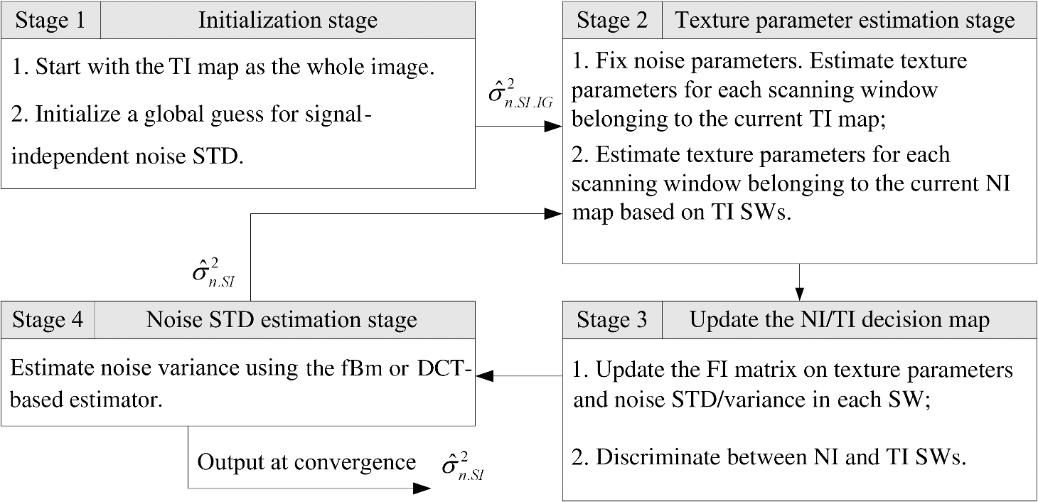
By saying “with as little variance as possible,” we mean that there is a certain theoretical limit on the estimation accuracy (in terms of standard deviation) of noise parameters from image data.15 It is desirable for an estimator to perform close to this limit. The true image content is certainly nonuniform and may include different texture patterns, edges, objects of small size, etc. All these heterogeneities should not essentially influence the performance of a noise parameter estimator; i.e., estimated bias and standard deviation should not increase significantly (over a theoretical limit). Potentially, the performance of blind methods can be very high—certainly higher than that of a human operator. The reason is that these methods can use subtler differences between image content and noise, which might be not visible to the human eye. But satisfying the above requirements altogether (and reaching a high level of estimation accuracy) for signal-dependent noise has been a difficult problem.12 Extended versions of approaches, originally proposed for the estimation of signal-independent noise standard deviation, have been considered to deal with signal-dependent noise, among them the well-known scatterplot approach.39 Recall that a scatterplot is a collection of points, each representing image local variance versus local mean. To reduce the influence of outliers, a robust fit to the scatterplot data points has typically been considered by different authors (e.g., Refs. 8, 10, and 39). Unfortunately, robust fit in the presence of a large percentage of abnormal local variance estimates (obtained from heterogeneous fragments) may appear very unstable. As a result, different fit strategies can lead to notably different estimation results.12 To meet all the requirements discussed above, we extend here the promising approach that we recently proposed in Ref. 15 to estimate the standard deviation (or variance) of signal-independent noise (assumed to be spatially uncorrelated). Our approach introduces two specific maps: the image texture informative (TI) map and the noise informative (NI) map. These two maps are complementary; i.e., for a given image, each scanning window (SW) belongs to one or another map. Assigning a given SW to one of these maps is decided based on the Fisher information (FI) on image texture parameters and noise standard deviation contained in this single window. In the NI map, a large amount of FI on the noise standard deviation is contained in each selected SW forming this map. Such SWs contribute in solving the main task, i.e., the accurate blind estimation of noise parameters. On the contrary, in the TI map, a large amount of FI on image texture parameters is contained in corresponding SWs. Such SWs are involved in solving an auxiliary task (i.e., the estimation of image texture parameters). Note that both tasks are not mutually exclusive since texture parameters for NI SWs and noise parameters for TI SWs remain unknown, due to mutual masking of texture and noise. Therefore, the core of our approach is to use both maps simultaneously in an iterative manner. Noise parameters are estimated from NI SWs and then are applied to improve the estimation accuracy of texture parameters from neighboring TI SWs. The latter parameters, in turn, are used to improve the estimation accuracy of noise parameters. To implement this scheme, we carry out the maximum likelihood (ML) estimation of a parametrical 2-D fractal Brownian motion (fBm) model, selected for describing locally the texture of a 2-D noisy image SW. The FI on the estimated parameter vector (including fBm-model parameters and noise standard deviation) can then be derived. To obtain the final estimation of noise standard deviation from the NI map, two alternatives, either fBm- or DCT-based estimators (, ), are proposed. The first one performs direct parametrical ML estimation of noise standard deviation from NI SWs, with a texture correlation matrix defined according to the fBm model and parameters derived from neighboring TI SWs. The second one applies DCT transform to NI SWs and uses only a fixed and limited number of high-frequency DCT coefficients to estimate noise standard deviation. Now, under signal-dependent noise hypothesis, the main difficulty is to take into account the variation of noise standard deviation with regard to image intensity (due to the signal-dependent noise component), while still resorting to image NI/TI maps. For this purpose, we analyze how image NI SWs are distributed over the intensity range. This distribution allows the finding of narrow intensity intervals where noise variance can be accurately estimated and the discarding of noninformative intensities (those without any NI SW detected). Final estimates of noise signal-independent/dependent component variances are obtained by linear fit applied to these accurate variance estimates localized with regard to intensity. The whole procedure ensures the absence of outliers among local estimates of noise variance. Therefore, robust fit procedures that can be unstable are no longer needed. This paper is organized as follows. Section 2 briefly introduces the fBm model and then recalls and signal-independent noise variance estimators that we previously proposed. Later in this section, the signal-dependent noise parameter estimation problem is introduced from an informational point of view, including FI distribution over the available intensity range for a given image. In Sec. 3, and estimators are extended for signal-dependent noise and the potential accuracy of such noise parameter estimates is provided. In Sec. 4, the performance of and estimators is comparatively assessed against two other modern methods in a large image database and real noise from a CCD sensor. Finally, in the last section, conclusions are offered. 2.Signal-Dependent Noise Parameters Estimation from Noise and TI Maps2.1.FBm Model for Describing Texture LocallyTo describe image texture locally, we propose to use the fBm model . Fractal analysis based on mathematical fBm processes has been suggested as a useful technique for characterizing real-life images, as they can describe quite complicated textures or shapes of natural scenes with a minimal parameter set.41 By definition, , , is a Gaussian process [the original coordinates are at the point (0,0): ] with the correlation function:42 In spatial terms, the Hurst exponent describes fBm-texture roughness ( for rough texture, for smooth),43 and describes fBm amplitude. By , , and , we denote a single-component image with columns and rows (for multi-component or color images, the approach proposed here should be applied component-wise). Suppose that the image is affected by signal-dependent noise according to the following model: where is the original noise-free image, is an ergodic Gaussian noise with zero mean, signal-dependent variance and a 2-D Dirac delta function for its spatial autocorrelation function. For a general case, for signal-dependent noise variance , we assume a polynomial model with degree : , where is true image intensity and is a coefficient vector of size .However, in the section of this paper that describes the experiment, we concentrate on a reduced-order noise model for recent CCD sensors. In this case, the noise is supposed to be the sum of two components: . The first one, , is signal-independent with variance , and the second one, , is signal-dependent with variance (Poisson-like noise). This corresponds to a polynomial model of the first order () and, thus the coefficient vector simply reduces to : 2.2.Structure of and Signal-Independent Noise Variance EstimatorsAt this point, let’s briefly recall the main ideas suggested in the and signal-independent noise variance estimators () proposed by the authors in Ref. 15. Their generalized structure is recalled in Fig. 1. This structure used the fBm model and both image NI and TI maps. In the estimation process, a processed sample corresponds to a noisy textural fragment or SW of the image. The sample is described by a statistical parametrical model. The model parameters vector includes both texture parameters (fBm-model parameters) and signal-independent noise variance . After initialization (stage 1), NI/TI maps and noise standard deviation are simply assumed to be equal to initial guesses or current refined estimates in stage 2. At this stage, texture parameters are estimated for each TI SW first. Then, these estimates act as texture parameter estimates in neighboring NI SWs. This stage results in estimates of the parameter vectors for all SWs for further use in stage 3. In stage 3, those SWs that can be efficiently used for estimating either noise or texture parameters are identified. We propose to perform this task by considering the corresponding FI on involved parameters or, equivalently the Cramér-Rao Lower Bound (CRLB), to each SW. By setting a proper threshold on CRLB, it becomes possible to find a subset of NI/TI SWs that provide noise/texture parameters estimates with a predefined accuracy. Finally, in stage 4, the noise standard deviation is estimated for each NI SW using either a fBm-model-based ML estimator () or DCT (). Note that by using only NI SWs ensures that all individual noise standard deviation estimates in stage 4 achieve a predefined accuracy and that there are no outliers among them. As a result, a simple nonrobust estimation procedure (for example, weighted mean) is sufficient in stage 4 to obtain the final estimate . 2.3.FI Distribution over ImagesWhen solving the estimation problem for signal-independent noise, the total amount of FI on noise standard deviation contained in all noise-informative SWs determines the potential performance of an estimator (in terms of its variance).15 For signal-dependent noise, when noise standard deviation is a function of true image intensity, the distribution of FI over the image intensity range becomes of major importance. Specifically, if all noise-informative SWs have the same intensity mean , only the value of can be estimated. This allows estimating the pure Poisson-like () or multiplicative () signal-dependent noise standard deviation by and , respectively (with accuracy that does not depend on ). If a mixture of signal-independent noise and either Poisson-like or multiplicative noise is assumed, the best accuracy can be achieved when FI is distributed equally between two intensities, and , with being as large as possible. When no a priori information about is available, then FI uniformly distributed over all image intensity ranges is the best option. Unfortunately, for a particular image, this distribution cannot be modified. What can be done, in practice, is to establish the actual distribution for a given image and to obtain the corresponding accuracy of noise parameter vector estimation, taking into account available a priori information. This problem will be addressed next, and and estimators will be extended to estimate the function. The corresponding FI about the parameter vector on texture parameters and noise standard deviation was introduced in Ref. 15 for a single SW () as where is information on fBm-model parameters, is information on signal-independent noise standard deviation, and is mutual information.Assume that noise-informative SWs have been detected, and assign mean intensity to the th NI SW. For the subset of these windows with , we assume a signal-independent noise model with standard deviation . Then, joint FI matrix on extended parameter vector can be obtained in a similar way: where . From the matrix , CRLB on can be found to be the corresponding element of the inverse matrix (marked by “” in the lower index below):Using , we define CRLB per unit intensity range as and relative CRLB per unit intensity range as where .To get better insight on the meaning of variables defined above, the possible shape of and its relation to the image content are illustrated in Fig. 2. Figure 2(a) displays the green component of image 3 from the NED2012 color images database (Noise Estimation Database), later referred to as the test image. We created the NED2012 database especially for testing the noise parameter estimator. It is described in detail in Sec. 4.1, later in this article. Fig. 2(a) Green component of image #3 from the NED2012 database; (b) relative CRLB per unit intensity range, , versus intensity for image #3 from the NED2012 database (test image) degraded with signal-dependent noise. 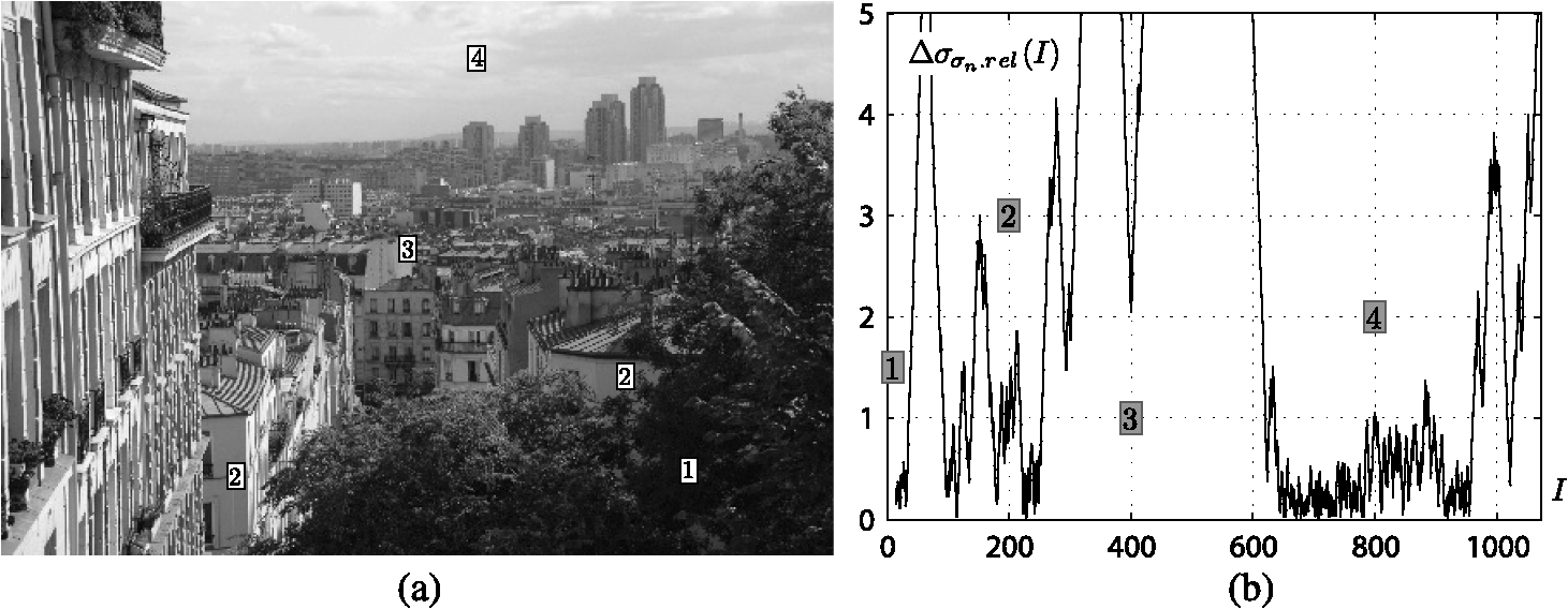 The function has been calculated for the test image, and it is displayed in Fig. 2(b). In this experiment, we fix to calculate . A way to calculate automatically will be described in Sec. 3.1. Intensities of the test image cover range approximately from 0 to 1,200. In Fig. 2(b), four image intensity intervals with the lowest can be seen, with image intensities around 10 (1), 200 (2), 400 (3), and 800 (4). Objects in the test image with intensities falling within intervals 1–4 are marked in Fig. 2(a) with the corresponding numbers. Interval 1 corresponds to the nonintensive dark tree texture, intervals 2 and 3 relate to homogeneous house fronts, and interval 4 relate to cloudy sky. One can see that indicates image areas that provide accurate noise standard deviation estimation and their localization with regard to image intensity. 3.and Estimators for Signal-Dependent Noise Parameters3.1.Preliminaries of the Proposed Estimators of Polynomial SD Noise VarianceWhile designing the signal-dependent noise parameter estimator, we assume piecewise-constant approximation to the function: where , , and , is the available image intensity range.As utilizing NI SWs along with either fBm-based or DCT-based noise standard deviation estimators ( or ) was proved to be efficient in Ref. 15 for signal-independent noise, we propose here to apply these two estimators to estimate in each NI SWs subset, with mean intensity falling within a given interval . Before using Eq. (8), the set of intervals should be properly selected. This can be done by taking into account the relationship between and . Indeed, for noninformative image intensities with high , the interval has to be increased to provide sufficiently accurate noise standard deviation estimates. Conversely, for informative image intensities with low (areas 1–4 in Fig. 2), the same accuracy can be achieved for smaller . It is natural to estimate noise standard deviation with a predefined accuracy for each considered intensity interval ; i.e., to require where is the center of interval . Eq. (9) is an extension of the thresholding procedure used in Ref. 15 to select a given SW as NI in the signal-independent noise case. Whereas this original constraint requires the signal-independent noise standard deviation to be estimated with a predefined accuracy from a single NI SW, Eq. (9) requires the same standard deviation estimation, but from the subset of NI SWs with mean intensities within the interval .According to Eq. (6), for an arbitrary intensity , equality in Eq. (9) holds for Therefore, is just a scaled-down version of . In the example considered in Fig. 2, we set . For this value, varies from 1 to 10 in informative intensity intervals 1–4 and exceeds 200 in noninformative intervals [shown by the peaks in Fig. 2(a)]. It follows that for informative intensities, noise variance can be accurately estimated from very narrow intensity intervals, enabling fine NLF analysis. Based on Eq. (10), the set of intervals is obtained by the following procedure:
For each interval , is estimated using either the or the estimator (under signal-independent hypothesis). At the same time, is calculated for future use. The output of the proposed signal-dependent noise estimator is the set of noise standard deviation estimates obtained for each interval and the corresponding set of mean intensities . Now, the maximum likelihood estimation (MLE) of coefficients vector is obtained by where is the Vandermonde matrix with elements , , and is the potential accuracy of the estimation of . The correlation matrix of the estimate has the following form: where is the true value of vector.3.2.Proposed Estimators of Polynomial SD Noise VarianceNote that the signal-dependent noise variance estimate obtained by Eq. (11) requires availability of the values of and , that are based on true noise variance . Therefore, the signal-dependent noise variance estimation procedure should operate iteratively as described below. The structure of the proposed estimator for texture parameters and signal-dependent noise standard deviation is summarized in Fig. 3. In the following, we provide a description of this estimator and illustrate its behavior based on the test image [Fig. 2(a)] for . True parameter vector is obtained for this image in the experiment via a calibration procedure (see Sec. 4.1 of this article for details). Fig. 3Generalized scheme of proposed and estimators for image texture and signal-dependent noise parameters. 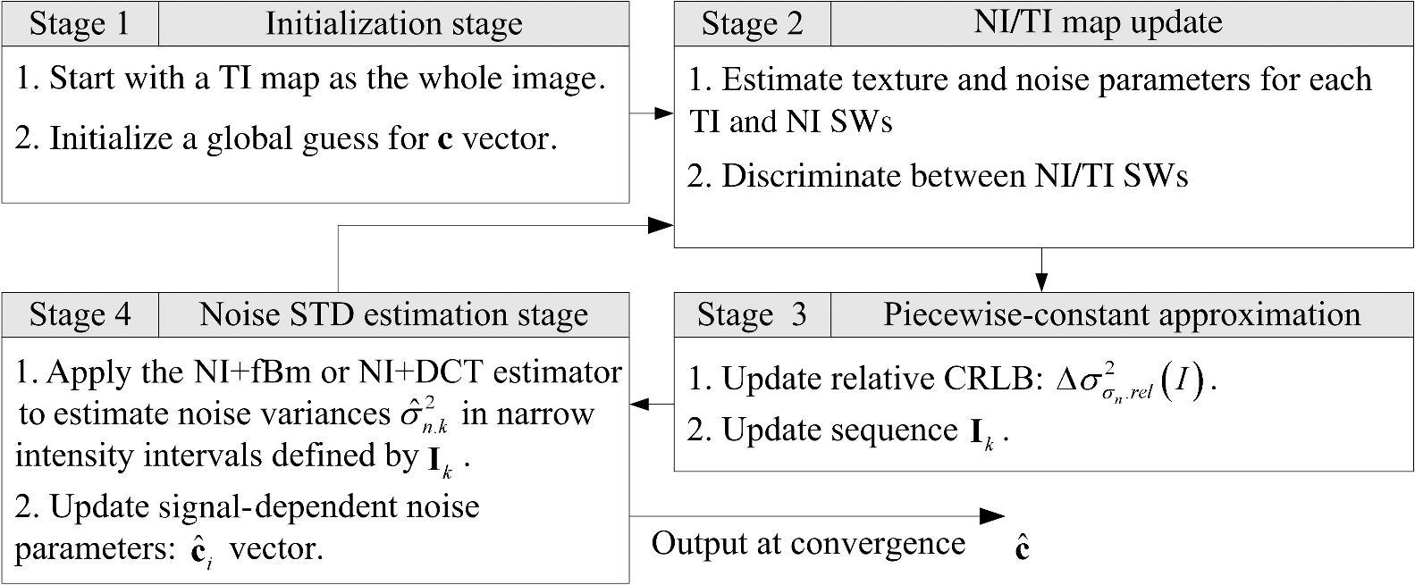 In the first stage, noise is assumed to be signal-independent and an initial guess is calculated as specified in Ref. 15. It is equal to the minimum of sample standard deviation estimates over all image nonoverlapping SWs. For the test image, the value was obtained. The initial guess for the vector assumes the initial value . Texture and noise parameter estimates and NI and TI maps are updated in stage 2. In this stage, we fix noise parameters to be equal to either an initial guess or the previously estimated value (here, defines the iteration index). The signal-dependent noise variance for each SW (both NI and TI) is calculated according to the retained polynomial noise model (a mixture of signal-independent and Poisson-like signal-dependent noises in this case) as , substituting true image intensity by mean intensity over current SW. Then, fBm-model parameters for TI and NI SWs are estimated, and discrimination between texture/NI SWs can be refined as specified in Ref. 15. Next, in stage 3, a current value of relative CRLB per unit image intensity () and the corresponding set of intervals are calculated as described above. For illustration purposes, the obtained in the first iteration is shown in Fig. 4(a) as a straight black line. Fig. 4Illustration of the signal-dependent noise estimation process by using the algorithm in Fig. 3 for the test image.  The set of intervals allows the estimating of values using either the fBm- or DCT-based estimator and refining the estimate according to Eq. (11). The estimates and function are both shown in Fig. 4(a) for the first iteration of the algorithm as black dots and a solid black line, respectively. The estimate is iteratively refined by repeating stages 2–4 until convergence. The convergence of the algorithm can be observed from the comparison of Fig. 4(a) with 4(b), where the first and the final (fifth) iteration estimates of , , and for the test image are shown. Note that for each iteration, Fig. 4 shows estimates at the beginning of the iteration (signal-independent noise for the first iteration), not at the end. It can be seen that estimates are concentrated at intensities where takes on minimal values. Noise variance estimate for from 600 to 1200 does not change significantly with iterations. Conversely, for from 0 to 300 that corresponds to areas (1) and (2) in Fig. 2(b), the noise variance estimate decreases from about 170 [the first iteration, Fig. 4(a)] to about 5 [the last iteration, Fig. 4(b)], and the number of estimates decreases significantly (a smaller number of SWs is considered NI by the algorithm). Now let us comment on the algorithm behavior for the textured area of the test image with an intensity close to 60 (dark trees in the lower-right part of the test image). With iterations, noise variance estimates are decreasing for this area. Consequently, the signal-to-noise ratio (measured locally) is constantly increasing. As a result, this area progressively becomes less and less noise informative [this is reflected by the increase of function clearly seen in Fig. 4]. Finally, in iteration 5 [Fig. 4(b)], this area is excluded from the noise variance estimation process (it becomes related to the TI map). The results obtained at final iteration confirm that, given a degraded image, indicates that image areas that can provide accurate noise variance estimation and their localization with regard to image intensity. It can be clearly seen that the estimated curve is very close to noise variance obtained by the calibration procedure. For the considered test image, there are enough NI intensities to provide a high estimation accuracy of signal-dependent noise variance. For images with not enough NI (homogeneous) areas for estimating noise parameters, may become inaccurate. Based on our experiments, we have found that this extreme case can always be detected by checking the accuracy of at the current iteration or the entries of the matrix [see Eq. (12) for details]. 4.Experimental Results Using the NED2012 DatabaseThis section deals with the application of the two designed estimators, and , of signal-dependent noise parameters to the NED2012 database of images that have been corrupted by signal-dependent noise. Estimator performance is analyzed and compared to that of the recently developed Automatic Scatterplot Reference Points Fitting with Restrictions (ASRPFR) method (discussed in Ref. 12) and the ClipPoisGaus_stdEst2D method published in Ref. 9. The primary goal of this study is to determine the potential accuracy of signal-dependent noise parameter estimation (variance of signal-independent and -dependent components) from real images of different types, and to compare the performance of existing estimators to this bound. 4.1.Image Database for Testing Signal-Dependent Noise Estimation Algorithms: NED2012A key item in testing noise variance estimators is the availability of images with known noise parameters. Artificial noise-free images with synthetic noise raise questions about the applicability of the obtained results to the real images corrupted by real noise. Another possibility lies in using real-life images with a low level of noise, with synthetic noise added for test purposes. In this area, the TID200844 database has been extensively used.45 However, we have identified four drawbacks of TID2008 that prevent us from exploiting it in our study:
To overcome these drawbacks, we have decided to base our study on 12-bit raw images from the Nikon D80 DSLR camera with a 10.2-Mpx CCD sensor. No extra noise was generated; we only dealt with the parameter estimation for noise that was originally present in D80 images. Our main assumption is that the noise parameters remain the same with time and camera operational conditions. Absence of noise spatial correlation is also assumed. Our experiments have shown no violation of these assumptions at the attained level of accuracy. To accurately estimate true noise parameters of Nikon D80 sensor for ISO100, we have used the following semi-automatic calibration procedure:
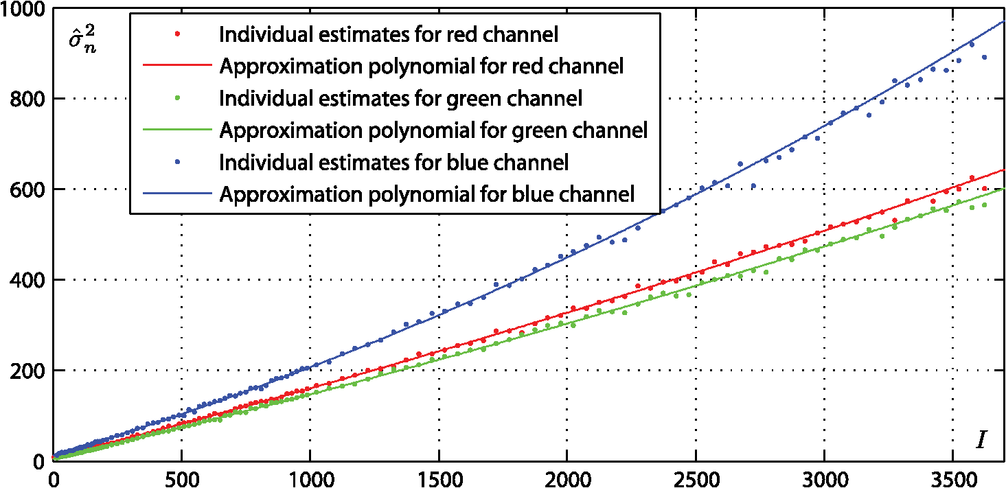
Visual analysis of noise variance dependence on image intensity shows notable deviation from the theoretic linear shape (first-order polynomial), especially for the blue component (Fig. 5). To take this into account, the order of the approximation polynomial was set to . The obtained estimates are given in Table 1 (we call them calibration lines). The noise parameters obtained via the calibration procedure will be marked with index “0” below. Table 1Sensor noise parameters for the Nikon D80 digital SLR camera (statistical error at one sigma level is specified)
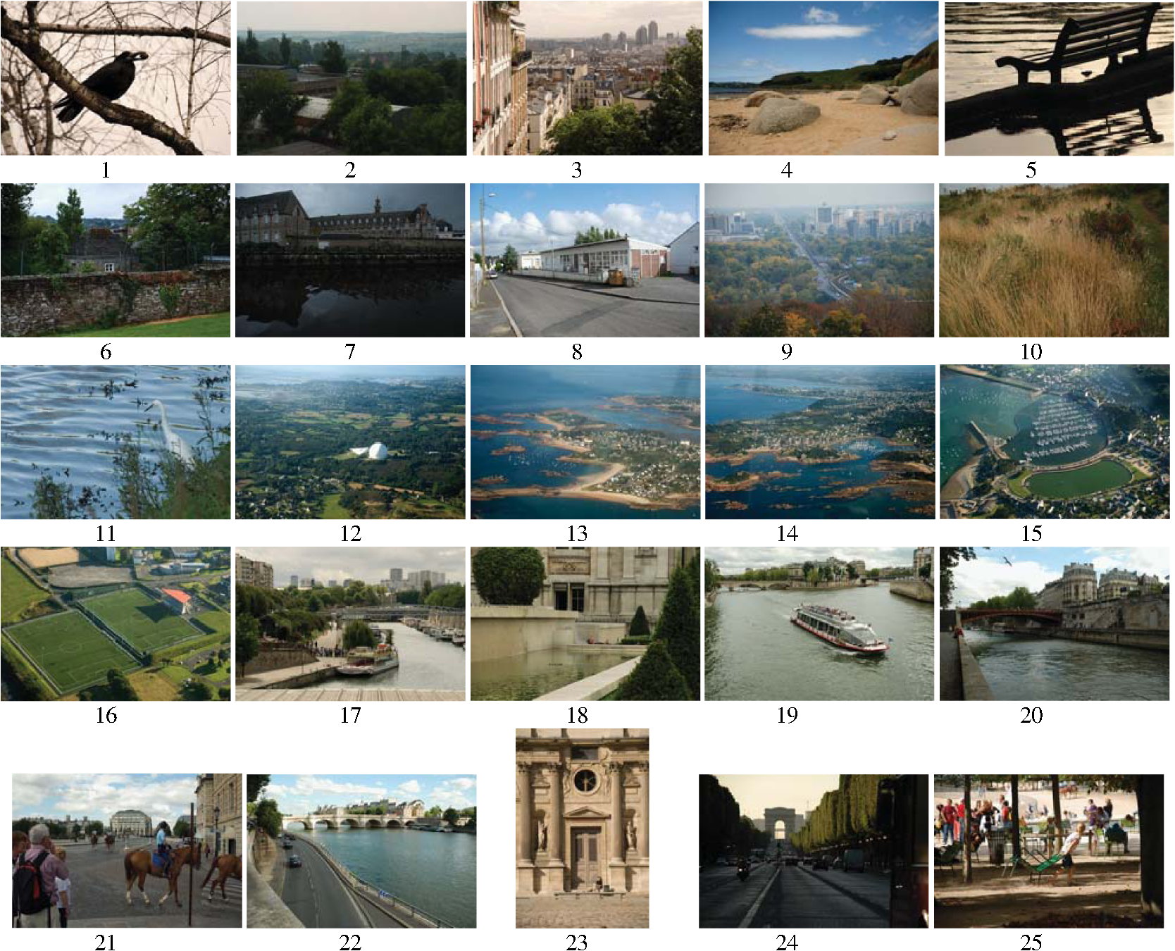
It can be seen that the green channel is the least noisy one, followed by the red and blue channels. Quadratic terms for all channels are nonzero. These values are statistically significant (more than or 14.3 sigma) and cannot be neglected. They probably appear due to the internal regulations of the camera. For testing the two proposed estimators, we selected 25 D80 images taken from the same camera during a two-year interval and organized them into the NED2012 database. The database includes images with different content. Some of them have large homogeneous areas (e.g., sky), while others are quite textural, and defocused areas are present (Fig. 6). All images are presented as a CFA array of in size. Red, green, and blue channel data were extracted from the CFA array by subsampling. Images have different ISO values (from 100 to 320), different shutter speeds (from to ), different apertures (from f/4 to f/14) and different focal lengths (from 18 mm to 135 mm). From this set of parameters, it is the ISO parameter that directly affects noise parameters for both signal-independent and -dependent components. In order to compensate for this influence and convert all images to the reference ISO100, we have simply normalized each image by a factor of 100/ISO before processing. We will first prove that estimation results obtained by the method agree with the calibration data shown above. For this goal, we applied the method to all images from the NED2012 database simultaneously by processing 1,500 SWs of randomly selected from each NED2012 image (a total of windows). In this manner, very high estimation accuracy of the , , and coefficients can be reached. Estimation results for all three channels are shown in Table 1 (the line). Figure 7 illustrates these results for the blue channel. Fig. 7Comparison of and calibration noise variance estimates for the blue channel of the NED2012 database. 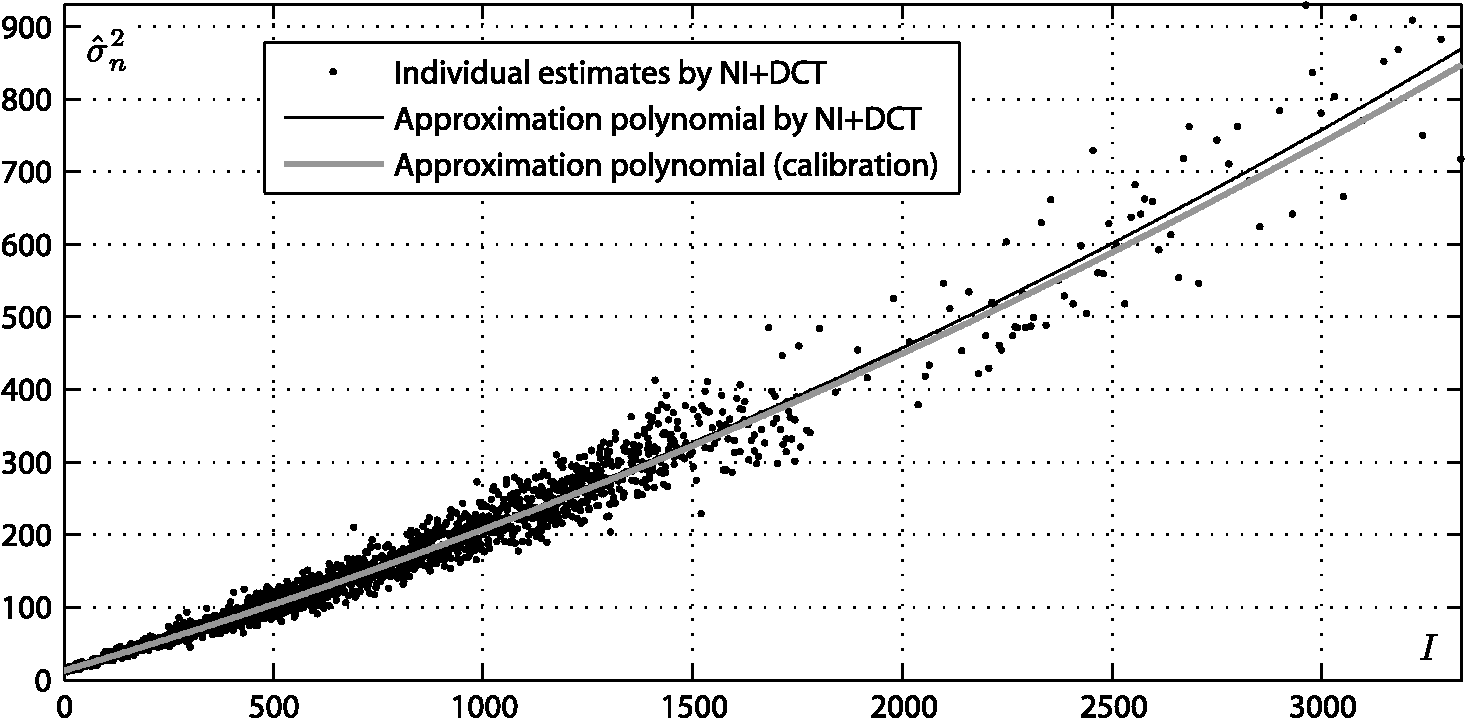 One can clearly see that there is no statistically significant difference between estimates of noise parameters obtained for two different datasets (the NED2012 database and the set of 17 calibration images) by the calibration procedure and the method (they differ by less than ). It is worth noting that the accuracy provided by the method is only slightly worse than the one obtained by the calibration procedure. In this test, the method shows its potential ability to deal with signal-dependent noise that is more complex than mixtures of additive and Poisson/multiplicative noises. In the next experiment, we restricted ourselves to the case of a mixture of signal-independent and Poisson-like signal-dependent noises. The overall noise variance is thus signal-dependent: . As was shown above, the noise in the Nikon D80 images does not strictly follow this linear model. Therefore, in order to nullify quadratic term before estimation, we normalized the image intensity in each SW by where is the mean of and , , and are taken from Table 1. After such normalization, noise parameters become as specified in Table 1, with .4.2.Accuracy Analysis of Signal-Dependent Noise Parameter EstimationThe considered set of four estimators, , , ASRPFR, and ClipPoisGaus_stdEst2D, were applied to each of the 25 images of the NED2012 database in a component-wise manner (red, green, and blue components were processed independently). A SW of in size was selected for both and . The choice of this particular SW size is justified in this subsection. For each component, the two noise variance components and were estimated. Overall, 25 estimates were obtained for each channel. Their empirical probability density functions (pdfs), pdf () and pdf (), are shown in Figs. 8 and 9, respectively. The main statistical characteristics of these estimates [mean , bias and standard deviation ] are given in Table 2. The bias measure is calculated as , where is the true value of . Fig. 8Experimental pdfs of signal-independent noise component variance estimates by (a) , (b) , (c) ASRPFR, and (d) ClipPoisGaus_stdEst2D. Calibration variances are marked by vertical dot-dashed lines. 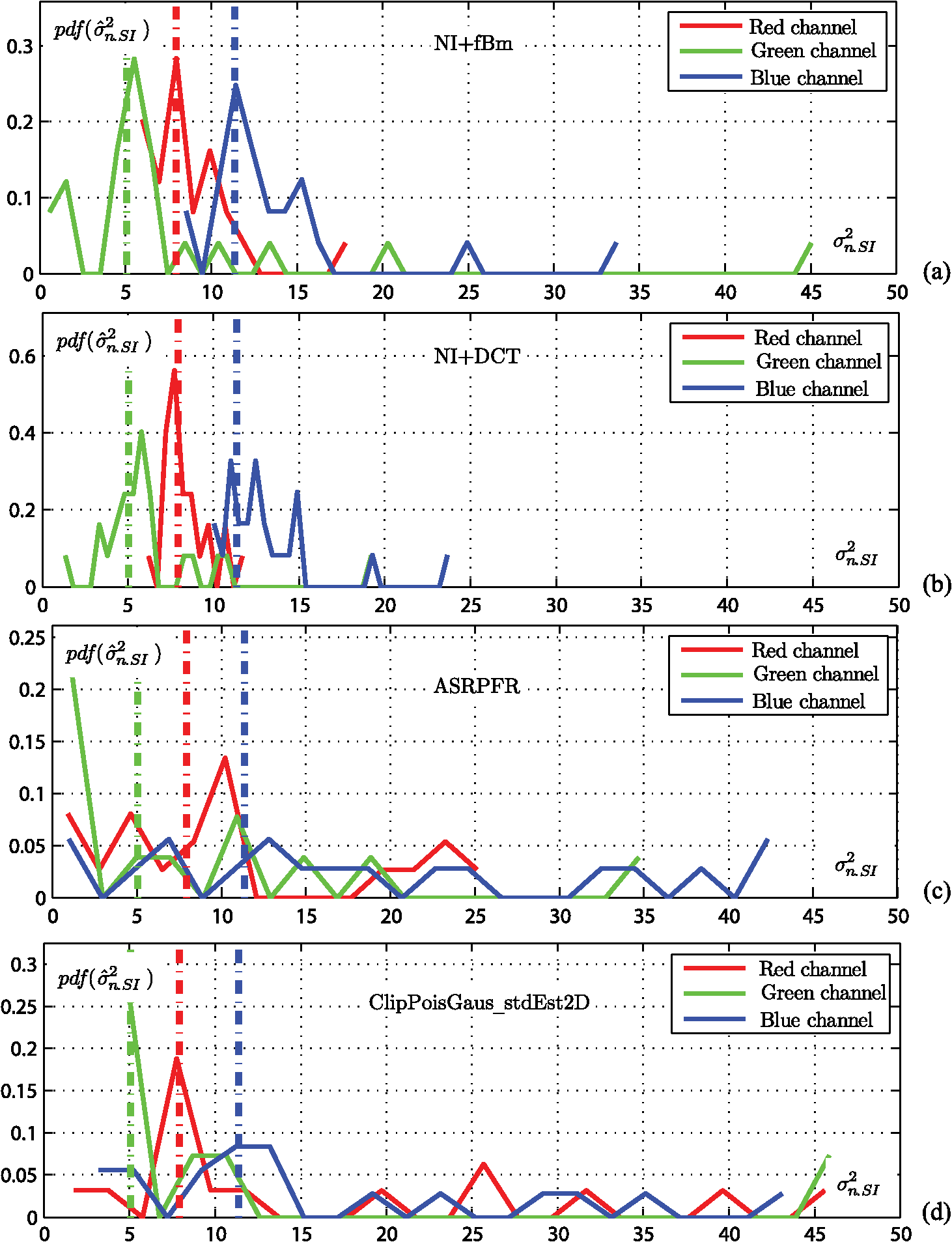 Fig. 9Experimental pdfs of signal-dependent noise component variance estimates by (a) , (b) , (c) ASRPFR, and (d) ClipPoisGaus_stdEst2D. Calibration variances are marked by vertical dot-dashed lines. 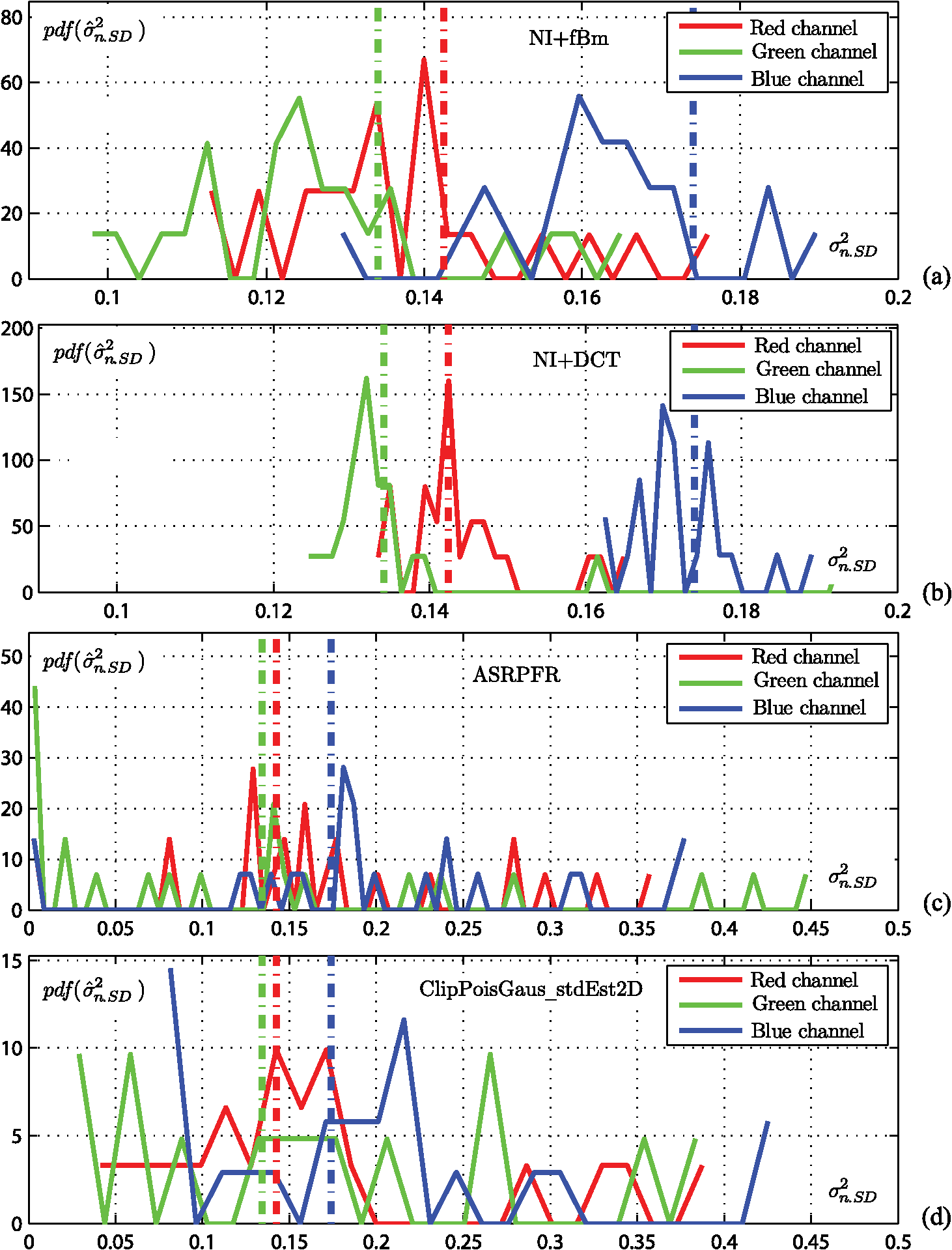 Table 2Mean value M(·), bias and standard deviation STD(·) of noise variance estimates on the NED2012 database.
Preliminary conclusions can be drawn from these results. Among these four estimators, ASRPFR and ClipPoisGaus_stdEst2D provide worse performance than the and with regard to both signal-independent and -dependent components. The main factor that degraded the performance of the ASRPFR and ClipPoisGaus_stdEst2D estimators is the significant number of outliers. However, they form a pronounced mode in the vicinity of the true value of signal-independent and -dependent noise component variances anyway. Therefore, we have decided to characterize the performance of these estimators by calling on extra robust measures. Specifically, median is used instead of mean value, and median absolute deviation (MAD) instead of standard deviation. Estimates of signal-independent noise component variance are biased for all four estimators. The absolute value of the bias is the smallest for the and methods (i.e., less than 6%). It increases to more than 30% for the ASRPFR method and to more than 12% for the ClipPoisGaus_stdEst2D. The estimates of the signal-dependent noise component variance are practically unbiased for the method, negatively biased by about 6% for the NI+fBm method, and exhibit a positive bias less than for the ASRPFR and ClipPoisGaus_stdEst2D methods. It is worth highlighting that the method provides the best estimation accuracy on both signal-independent and -dependent components. More precisely, with regard to the standard deviation of the noise variance estimates (specified in Table 2), it outperforms the method by approximately 1.25 to 2.6 times, the ASRPFR method by 3.6 to 10 times, and by an even greater degree for the ClipPoisGaus_stdEst2D. We explain the reduced performance of the estimator with regard to the one by the sensitivity of the former to errors on Hurst exponent estimation. A second possible reason could be deviations of real image texture from the assumed fBm-model. It is important to mention here that both ASRPFR and ClipPoisGaus_stdEst2D have been applied to NED2012 images without normalization [Eq. (13)] for quadratic term compensation. The reason for this is that such normalization operates at the SW level and depends on image partitioning during processing. We had no opportunity to modify the original implementation of ASRPFR and ClipPoisGaus_stdEst2D to take this into account. Therefore, in an additional experiment, we quantified the noncompensated term influence on (Table 2). Overall, it led to negative bias of signal-independent component variance and positive bias of signal-dependent component variance. For red and green channels, this additional bias was negligible and does not exceed 5% in magnitude. For the blue channel, this bias was more significant, with a magnitude of about 15%. We thus believe this is evidence that the noncompensated term cannot explain the decreased performance of ASRPFR and ClipPoisGaus_stdEst2D. In Fig. 10, we detail the signal-independent and -dependent noise variance estimates obtained with the best estimator on each component (red, green, and blue) of all images from the NED2012 database. For most of the images, very accurate estimates were obtained. For these images, the potential estimation accuracy on the signal-independent noise component variance is about 0.2–1, and it is about on the signal-independent noise component variance. But for some of the images, namely 13, 15, 16, 22, and 23, an increased estimation error was observed. This is reflected by a corresponding increase in the potential estimation accuracy for signal-independent and -dependent noise components to about 2 and , respectively. Fig. 10(a) Signal-independent and (b) signal-dependent noise component variance according to image index estimated by the on red, green, and blue components of each image from the NED2012 database. The true noise parameters are shown as dashed horizontal lines.  Let us now assess the efficiency of the analyzed estimators with regard to the diagonal terms of the correlation matrix of coefficient vector defined above by Eq. (12). For this purpose, two normalized errors, one for and another one for , respectively, are to be considered: Note that for an efficient estimator, both and should be distributed close to the normal distribution . The statistical efficiency of the analyzed estimators with regard to these bounds can be estimated as where XX is the noise component label (either SI or SD), and the sum for each estimator is calculated in Eq. (14) over all available estimates.Figure 11 displays and pdfs, respectively, for the best method (with ). The theoretical pdf is added for comparison purposes. Efficiencies for both noise components are shown in Table 3 for four different window sizes: , 9, 11, and 13. Fig. 11Empirical pdfs of the normalized estimates of signal-independent and signal-dependent noise components variances by the estimator . The theoretical pdf is shown as a dashed black curve. 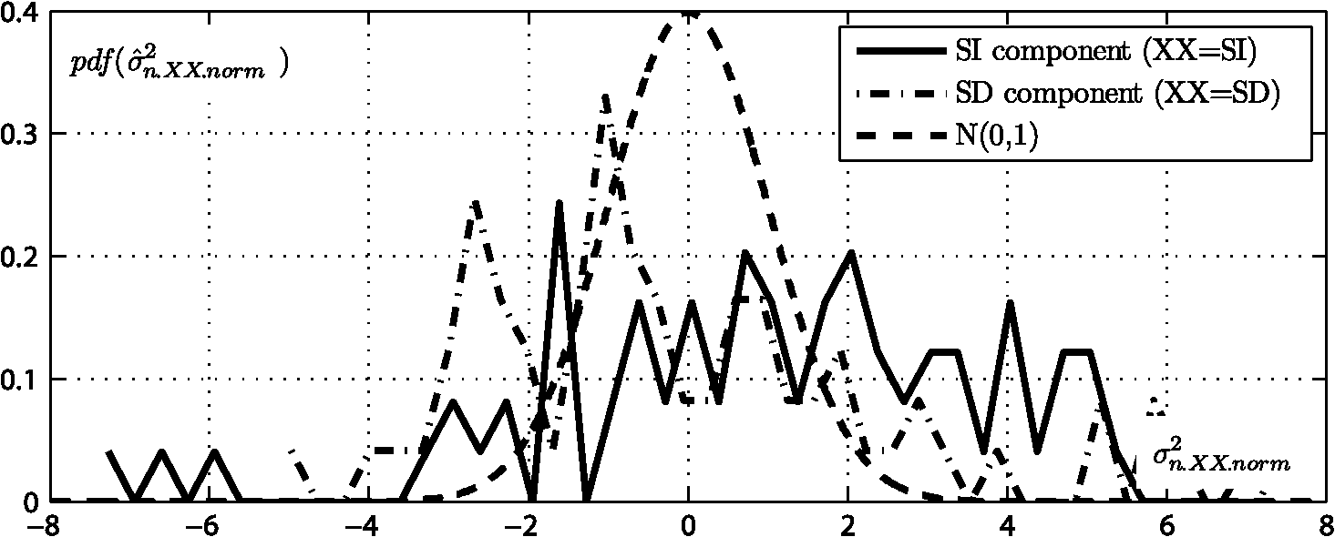 Table 3Statistical characteristics of normalized estimates for the NED2012 database (tree channels).
As is shown, the estimator exhibits rather high efficiency for different SW sizes, with a value of about 10 for both noise components. Note that for the estimator, the corresponding efficiency (not included in Table 3) is about 2%, and it is less than 0.1% for both the ASRPFR and ClipPoisGaus_stdEst2D estimators. More detailed analysis shows that the performance of the estimator is highest for and 11. It is slightly degrading for and the degradation is much more significant for . This can be explained by the influence of two factors compensating each other. On one side, the accuracy of texture parameter estimation reduces for smaller sized SWs. This factor is responsible for the decline in performance for . On the other hand, the image texture becomes more heterogeneous for larger windows, making the fBm model less adequate. This factor is responsible for the slight decrease in performance for . Taking into account that the processing time is increasing fast with the SW size, we suggest as the best setting. It is important to note that even for the estimator, there exists an essential gap between the current level of accuracy and potential accuracy . This gap can be attributed equally to inherent shortcomings of the estimator and to the bound itself. For example, the latter does not properly take into account errors associated with Hurst exponent interpolation from TI map to NI map. Further research needs to be undertaken to reduce this gap and to better assess the potential of blind noise parameter estimation. 5.ConclusionsThe problem of parameter estimation of signal-dependent noise has been considered in this paper. It has been shown that distribution of FI with regard to noise standard deviation over the available image intensity range is mainly responsible for the accuracy of signal-dependent noise parameter estimation. This is in contrast to signal-independent noise, for which estimation accuracy is defined by overall FI. This feature has been utilized to extend the and estimators previously proposed by the authors to the case of signal-dependent noise. The performance of the and estimators has been assessed using the newly developed NED2012 database, with real noise originating from the CCD sensor. True values of noise parameters in images from the NED2012 database have been found via the calibration procedure. For images from the NED2012 database, the proposed and estimators are shown to notably outperform the recently published ASRPFR and ClipPoisGaus_stdEst2D estimators. Between these two estimators, is considerably more effective than in terms of bias and variance of noise parameter estimates. Overall estimation accuracy of signal-dependent noise parameters for images of the NED2012 database is high: estimates are slightly biased most of the time, with a bias value of less than 2% and a standard deviation of about 10% to 25% with regard to true noise parameter value. However, for some images with complex content, component-wise processing fails to provide sufficiently accurate results. The distinctive feature of our approach is its ability to calculate the potential estimation accuracy of signal-dependent noise parameters for a given noisy image. We have found that there exists an essential gap between the obtained accuracy with the best estimator and the potential estimation accuracy thus provided ( statistical efficiency is about 10%). Such a gap indicates the necessity of further research in this area to design more efficient estimators and to obtain a more accurate lower bound on the performance of such estimators. In general, the proposed estimation algorithms (preferably the estimator) can be used for blind evaluation of an arbitrary polynomial dependency of the noise standard deviation on image intensity. Such experiments for second-order polynomials have been successfully carried out. In all cases, the potential estimation accuracy of polynomial coefficients can be obtained. AcknowledgmentsHere, we would like to thank S. Abramov for passing us results for the ASRPFR estimator and A. Foi for discussions, assistance and making implementation of his method available at http://www.cs.tut.fi/~foi/sensornoise.html. This work has been partly supported by the French-Ukrainian program Dnipro (PHC DNIPRO 2013, Projet No. 28370QL). ReferencesB. Vozelet al.,
“Blind determination of noise type for spaceborne and airborne remote sensing,”
Multivariate Image Processing, 263
–302 Wiley-ISTE, London, United Kingdom
(2009). Google Scholar
A. AmerE. Dubois,
“Fast and reliable structure-oriented video noise estimation,”
IEEE Trans. Circuits Syst. Video Technol., 15
(1), 113
–118
(2005). http://dx.doi.org/10.1109/TCSVT.2004.837017(410) 1 ITCTEM 1051-8215 Google Scholar
Y.-H. KimJ. Lee,
“Image feature and noise detection based on statistical hypothesis tests and their applications in noise reduction,”
IEEE Trans. Consum. Electron., 51
(4), 1367
–1378
(2005). http://dx.doi.org/10.1109/TCE.2005.1561869 ITCEDA 0098-3063 Google Scholar
G. Messinaet al.,
“Fast method for noise level estimation and integrated noise reduction,”
IEEE Trans. Consum. Electron., 51
(3), 1028
–1033
(2005). http://dx.doi.org/10.1109/TCE.2005.1510518 ITCEDA 0098-3063 Google Scholar
C. StaelinH. Nachlieli,
“Image noise estimation using color information,”
(2007). Google Scholar
A. Boscoet al.,
“Fast noise level estimation using a convergent multiframe approach,”
in Proc. IEEE Int. Conf. on Image Process.,
2621
–2624
(2006). Google Scholar
S. H. Lim,
“Characterization of noise in digital photographs for image processing,”
Proc. SPIE, 6069 60690O
(2006). http://dx.doi.org/10.1117/12.655915 Google Scholar
V. V. Lukinet al.,
“Improved minimal inter-quantile distance method for blind estimation of noise variance in images,”
Proc. SPIE, 6748 67481I
(2007). http://dx.doi.org/10.1117/12.738006 Google Scholar
A. Foiet al.,
“Practical Poissonian-Gaussian noise modelling and fitting for single-image raw-data,”
IEEE Trans. Image Process., 17
(10), 1737
–1754
(2008). http://dx.doi.org/10.1109/TIP.2008.2001399 IIPRE4 1057-7149 Google Scholar
C. Liuet al.,
“Automatic estimation and removal of noise from a single image,”
IEEE Trans. Pattern Anal. Mach. Intell., 30
(2), 299
–314
(2008). http://dx.doi.org/10.1109/TPAMI.2007.1176 ITPIDJ 0162-8828 Google Scholar
A. Boscoet al.,
“Signal-dependent raw image denoising using sensor noise characterization via multiple acquisitions,”
Proc. SPIE, 7537 753705
(2010). http://dx.doi.org/10.1117/12.838608 Google Scholar
S. Abramovet al.,
“Methods for blind estimation of the variance of mixed noise and their performance analysis,”
Numerical Analysis—Theory and Application, 49
–70 InTech, Rijeka, Croatia
(2011). Google Scholar
V. V. Lukinet al.,
“Methods and automatic procedures for processing images based on blind evaluation of noise type and characteristics,”
J. Appl. Remote Sens., 5
(1), 053502
(2011). http://dx.doi.org/10.1117/1.3539768 1931-3195 Google Scholar
J. Meolaet al.,
“Modeling and estimation of signal-dependent noise in hyperspectral imagery,”
Appl. Opt., 50
(21), 3829
–3846
(2011). http://dx.doi.org/10.1364/AO.50.003829 APOPAI 0003-6935 Google Scholar
M. Usset al.,
“Image informative maps for estimating noise standard deviation and texture parameters,”
EURASIP J. Adv. Signal Process., 2011 806516
(2011). http://dx.doi.org/10.1155/2011/806516 Google Scholar
P. Milanfar,
“A tour of modern image filtering: new insights and methods, both practical and theoretical,”
IEEE Signal Process. Mag., 30
(1), 106
–128
(2013). https://doi.org/http://dx.doi.org10.1109/MSP.2011.2179329 Google Scholar
D. T. Kuanet al.,
“Adaptive noise smoothing filter for images with signal-dependent noise,”
IEEE Trans. Pattern Anal. Mach. Intell., PAMI-7
(2), 165
–177
(1985). http://dx.doi.org/10.1109/TPAMI.1985.4767641 ITPIDJ 0162-8828 Google Scholar
H. FarajiJ. MacLean,
“Adaptive suppression of CCD signal-dependent noise in light space,”
in Proc. IEEE Int. Conf. on Acoustics, Speech, and Signal Process.,
iii-217
–220
(2004). Google Scholar
K. HirakawaT.W. Parks,
“Image denoising for signal-dependent noise,”
in Proc. IEEE Int. Conf. on Acoustics, Speech, and Signal Process.,
29
–32
(2005). Google Scholar
M. Pesensonet al.,
“Filtering of signal-dependent noise applied to MIPS data,”
in Proc. Astronomical Data Analysis Software and Systems XIV,
483
–486
(2005). Google Scholar
F. ArgentiG. TorricelliL. Alparone,
“MMSE filtering of generalised signal-dependent noise in spatial and shift-invariant wavelet domains,”
Signal Process., 86
(8), 2056
–2066
(2006). http://dx.doi.org/10.1016/j.sigpro.2005.10.014 SPRODR 0165-1684 Google Scholar
B. GoossensA. PizuricaW. Philips,
“Wavelet domain image denoising for non-stationary noise and signal-dependent noise,”
in Proc. IEEE Int. Conf. on Image Process.,
1425
–1428
(2006). Google Scholar
A. Foiet al.,
“Adaptive-size block transforms for signal-dependent noise removal,”
in Proc. 7th Nordic Signal Process. Symposium,
94
–97
(2006). Google Scholar
R. Oktemet al.,
“Locally adaptive DCT filtering for signal-dependent noise removal,”
EURASIP J. Adv. Signal Process., 2007 42472
(2007). http://dx.doi.org/10.1155/2007/42472 Google Scholar
T. Saitoet al.,
“Removal of signal-dependent noise for a digital camera,”
Proc. SPIE, 6502 65020E
(2007). http://dx.doi.org/10.1117/12.702980 Google Scholar
S. Nakamoriet al.,
“Filtering in generalized signal-dependent noise model using covariance information,”
Math. Comp. Model., E91-A
(3), 809
–817
(2008). http://dx.doi.org/10.1093/ietfec/e91-a.3.809 MCMOEG 0895-7177 Google Scholar
M. J. García-Ligeroet al.,
“Derivation of linear estimation algorithms from measurements affected by multiplicative and additive noises,”
J. Comp. Appl. Math., 234
(3), 794
–804
(2010). http://dx.doi.org/10.1016/j.cam.2010.01.043 JCAMDI 0377-0427 Google Scholar
B. Aiazziet al.,
“Benefits of signal-dependent noise reduction for spectral analysis of data from advanced imaging spectrometers,”
in Proc. 3rd Workshop on Hyperspectral Image and Signal Process.: Evolution in Remote Sens.,
1
–4
(2011). Google Scholar
P. ChatterjeeP. Milanfar,
“Is denoising dead?,”
IEEE Trans. Image Process., 19
(4), 895
–911
(2010). http://dx.doi.org/10.1109/TIP.2009.2037087 IIPRE4 1057-7149 Google Scholar
P. ChatterjeeP. Milanfar,
“Practical bounds on image denoising: From estimation to information,”
IEEE Trans. Image Process., 20
(5), 1221
–1233
(2011). http://dx.doi.org/10.1109/TIP.2010.2092440 IIPRE4 1057-7149 Google Scholar
V. Lukinet al.,
“Image filtering: Potential efficiency and current problems,”
in Proc. ICASSP’11,
1433
–1436
(2011). Google Scholar
F. D. Van Der MeerS. M. Dejong, Imaging Spectrometry: Basic Principles and Prospective Applications, 35
–38 Kluwer, Dordrecht, the Netherlands
(2001). Google Scholar
L. SendurI.W. Selesnick,
“Bivariate shrinkage with local variance estimation,”
IEEE Signal Process. Lett., 9
(12), 438
–441
(2002). http://dx.doi.org/10.1109/LSP.2002.806054 IESPEJ 1070-9908 Google Scholar
N. N. Ponomarenkoet al.,
“A method for blind estimation of spatially correlated noise characteristics,”
Proc. SPIE, 7532 753208
(2010). http://dx.doi.org/10.1117/12.847986 Google Scholar
D. ZoranY. Weiss,
“Scale invariance and noise in natural images,”
in Proc. IEEE 12th Int. Conf. Comput. Vis.,
2209
–2216
(2009). Google Scholar
N. N. Ponomarenkoet al.,
“Blind evaluation of additive noise variance in textured images by nonlinear processing of block DCT coefficients,”
Proc. SPIE, 5014 178
–189
(2003). http://dx.doi.org/10.1117/12.477717 Google Scholar
L. SendurI.W. Selesnick,
“Bivariate shrinkage with local variance estimation,”
IEEE Signal Process. Lett., 9
(12), 438
–441
(2002). http://dx.doi.org/10.1109/LSP.2002.806054 IESPEJ 1070-9908 Google Scholar
A. De StefanoP. R. WhiteW. B. Collis,
“Training methods for image noise level estimation on wavelet components,”
EURASIP J. Appl. Signal Process., 2004
(16), 2400
–2407
(2004). http://dx.doi.org/10.1155/S1110865704401218 1110-8657 Google Scholar
L. Alparoneet al.,
“Quality assessment of data products from a new generation airborne imaging spectrometer,”
in Proc. IEEE Int. Geosci. and Remote Sens. Symposium,
IV-422
–IV-425
(2009). Google Scholar
Y. TsinV. RameshT. Kanade,
“Statistical calibration of CCD imaging process,”
in Proc. 8th IEEE Int. Conf. Comput. Vis.,
480
–487
(2001). Google Scholar
B. Pesquet-PopescuJ. L. Véhel,
“Stochastic fractal models for image processing,”
IEEE Signal. Process. Mag., 19
(5), 48
–62
(2002). http://dx.doi.org/10.1109/MSP.2002.1028352 Google Scholar
P. Flandrin,
“On the spectrum of fractional Brownian motions,”
IEEE Trans. Inform. Theor., 35
(1), 197
–199
(1989). http://dx.doi.org/10.1109/18.42195 IETTAW 0018-9448 Google Scholar
A. P. Pentland,
“Fractal-based description of natural scenes,”
IEEE Trans. Patt. Anal. Mach. Intell., PAMI-6
(6), 661
–674
(1984). http://dx.doi.org/10.1109/TPAMI.1984.4767591 ITPIDJ 0162-8828 Google Scholar
N. Ponomarenkoet al.,
“Color image database for evaluation of image quality metrics,”
in Proc. IEEE Workshop on Multimedia Signal Process.,
403
–408
(2008). Google Scholar
V. Lukinet al.,
“Testing of methods for blind estimation of noise variance on large image database,”
Theoretical and Practical Aspects of Digital Signal Processing in Informational-Telecommunication Systems, South-Russian State University of Economics and Service, Shakhty, Russia
(2009). Google Scholar
Biography Mykhail L. Uss graduated from National Aerospace University (Ukraine) in 2002 and got a diploma with honor in radio engineering. Since then, he has been with the Department of Aircraft Radioelectronic Systems Design of National Aerospace University. He obtained the Candidate of Technical Science degree in DSP for remote sensing from National Aerospace University (Ukraine) in 2006, and then a PhD from the University of Rennes in France in 2011. Currently, he is head of the Department of Aircraft Radioelectronic Systems Design. His research interests include the statistical theory of radio-technical systems, digital signal/image processing, blind estimation of noise characteristics, and theory of fractal sets with applications to image processing and remote sensing.  Benoit Vozel obtained the State Engineering degree and the MSc degree in control and computer science from École Centrale de Nantes (France) in 1991, and then a PhD from the same university in 1994. As a PhD student, he was with the Signal Processing Group at Institut de Recherche en Communication et Cybernétique de Nantes, where he worked on the detection of abrupt changes in signals. Since 1995, he has been with the Engineering School of Applied Sciences and Technology, University of Rennes in France, where he is currently working in the Signal and Multicomponent/Multimodal Image Processing Laboratory. His research interests generally concern blind estimation of noise characteristics, image filtering and restoration, and adaptive image and remote sensing data processing.  Vladimir V. Lukin graduated from Kharkov Aviation Institute (now National Aerospace University, Ukraine) in 1983 and got a diploma with honors in radio engineering. Since then, he has been with the Department of Transmitters, Receivers, and Signal Processing of National Aerospace University. He defended the thesis of Candidate of Technical Science in 1988 and the thesis of Doctor of Technical Science in 2002 in DSP for remote sensing. Since 1995, he has been in cooperation with Tampere University of Technology. Currently, he is the department’s vice chairman. His research interests include digital signal/image processing, remote sensing data processing, and image filtering and compression.  Kacem Chehdi received the PhD and “Habilitation à diriger des recherches” degrees in signal processing and telecommunications from the University of Rennes in France in 1986 and 1992, respectively. He is currently with the University of Rennes, where he was an assistant professor from 1986 to 1992, has been a professor of signal and image processing with the Engineering School of Applied Sciences and Technology since 1993, has been the head of the Signal and Multicomponent/Multimodal Image Processing Laboratory (TSI2M) since 2004, and was the head of the Analysis Systems of Information Processing Laboratory from 1998 to 2003. His research interests include adaptive processing at every level in the pattern recognition chain by vision, blind restoration, and blind filtering (in particular, the identification of the physical nature of image degradations and the development of adaptive algorithms), and segmentation and registration topics (in particular, the development of unsupervised, cooperative, and adaptive systems). The main applications currently under investigation are multispectral and hyperspectral image processing and analysis. |
|||||||||||||||||||||||||||||||||||||||||||||||||||||||||||||||||||||||||||||||||||||||||||||||||||||||||||||||||||||||||||||||||||||||||||||||||||||||||||||||||||||||||||||||||||||||||||||||||||||||||||||||||||||||||||||||||||||||||||||||||||||||||||||||||||||||||||||||||||||||||||||||||||||||||||||||||