

|
|
1.IntroductionNoninvasive cardiac imaging is an invaluable tool for the diagnosis and treatment of cardiovascular disease (CVD). Magnetic resonance imaging (MRI), computed tomography (CT), positron emission tomography (PET), single photon emission computed tomography (SPECT), and ultrasound (US) have been used extensively for physiologic understanding and diagnostic purposes in cardiology. These imaging technologies have greatly increased our understanding of normal and diseased anatomy. Cardiac image segmentation plays a crucial role and allows for a wide range of applications, including quantification of volume, computer-aided diagnosis, localization of pathology, and image-guided interventions. However, manual delineation is tedious, time-consuming, and is limited by inter- and intraobserver variability. In addition, many segmentation algorithms are sensitive to the initialization and therefore the results are not always reproducible, which is also limited by interalgorithm variability. Furthermore, the amount and quality of imaging data that needs to be routinely acquired in one or more subjects has increased significantly. Therefore, it is crucial to develop automated, precise, and reproducible segmentation methods. Figure 1 illustrates an example of segmentation of heart on CT scan. Fig. 1An example of heart chamber segmentation in 3-D contrast CT volumes with green line delineation for the LV endocardium, magenta for the LV epicardium, cyan for the left atrium (LA), orange for the right ventricle (RV), and blue for the right atrium (RA).1 The first row shows a full torso view (the first column) and the closeup view (the right three columns) of three orthogonal cuts from 3-D volume data. The four images in the second row show the tracking results for the heart chambers on a dynamic 3-D sequence with 10 frames. (Reproduced from Y. Zheng et al. with permission of ©2008 IEEE.) 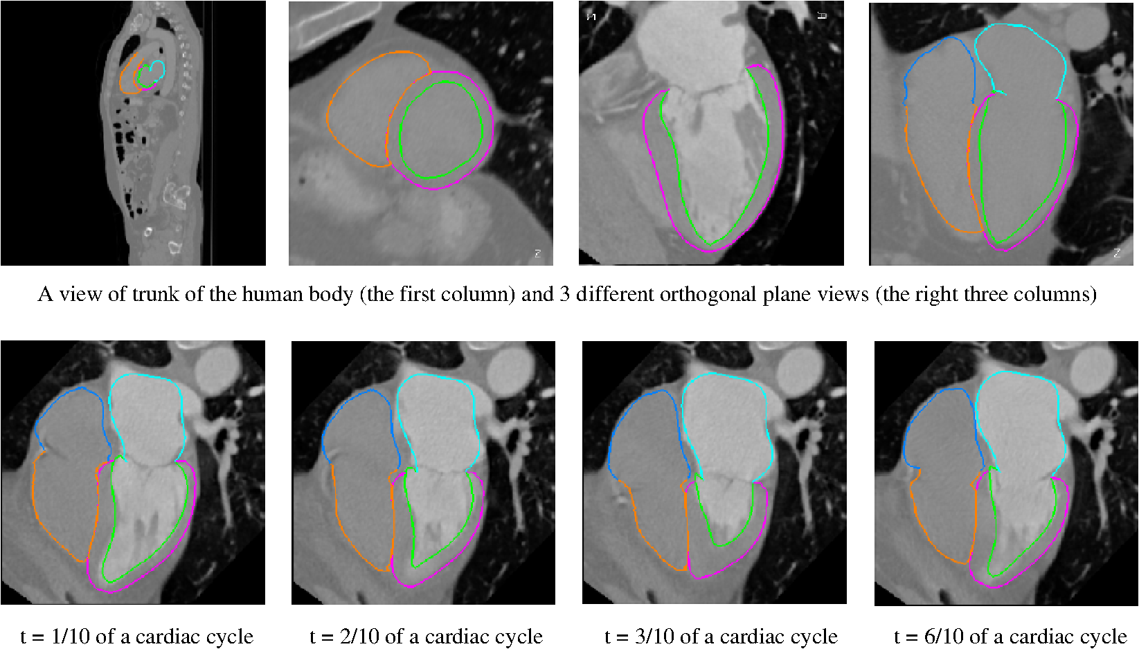 A variety of segmentation techniques have been proposed over the last few decades. While earlier approaches were often based on heuristics, recent studies employ more sophisticated and principled techniques. However, cardiac image segmentation still remained a challenge due to the highly variable nature of cardiac anatomy, function, and pathology.2 Furthermore, intensity distributions are heavily influenced by the disease state, imaging protocols, artifacts, or noise. Therefore, many researchers are seeking techniques to deal with such constraints. The research in cardiac image segmentation ranges from the fundamental problems of image analysis, including shape modeling and tracking, to more applied topics such as clinical quantification, computer-aided diagnosis, and image-guided interventions. In this review, we aim to provide an overview on cardiac segmentation methods applied to images from major noninvasive modalities such as US, PET/SPECT, CT, and MRI. We focus on the segmentation of the cardiac chambers and whole heart applied to static and gated images (obtained through the cardiac cycle). In addition, we also discuss important clinical applications, characteristics of imaging modalities, and validation methods used for cardiac segmentation. We do not discuss coronary vessel tracking, which is a separate topic. We hope that this article can serve as a useful guide to recent developments in this growing field. The review is organized as follows. The clinical background of cardiac image segmentation is discussed in Sec. 2. Numerous segmentation methods are described in Sec. 3. Cardiac imaging modalities are reviewed in Sec. 4. Approaches to validation of the segmentation results are discussed in Sec. 5. Concluding remarks are given in Sec. 6. 2.Clinical BackgroundCVD is the major cause of morbidity and mortality in the western world. More than 2,200 patients die of CVD each day in the United States alone.3 CVD involves a variety of disorders of the cardiac muscle and the vascular system. The common causes of CVD include ischemic heart disease and congestive heart failure.4 Cardiac imaging has played a crucial and complementary role to the diagnosis and treatment of patients with known or suspected CVD. In the case of ischemic heart disease, the first consequence of the disease is the changes in the myocardial perfusion assessed by SPECT and PET or by MRI.5 In particular, the perfusion deficit leads to metabolic changes in myocardial tissues assessed by PET. A myocardial ischemia could further diminish ejection of blood because of the reduced capacity of the heart as analyzed by the myocardial contractile function using US, PET/SPECT, CT, or MRI. Assessment of the left ventricle (LV) contractile function is essential for diagnosis and prognosis of CVD. The LV contractile function is commonly analyzed as it pumps oxygenated blood to the entire body.6,7 The computer-aided or fully automated segmentation of the ventricular myocardium is generally used to standardize analysis and improve the reproducibility of the assessment of contractile cardiac function.8 In addition, it forms an important preliminary step to provide useful diagnostic information by quantifying clinically important parameters, including end-diastolic volume (EDV), end-systolic volume (ESV), ejection fraction (EF), wall motion and thickening, wall thickness, stroke volume (SV), and transient ischemic dilation (TID).9 Furthermore, segmentation of the LV is necessary for the quantification of myocardial perfusion,10 the size of the myocardial infarct,11 or myocardial mass.12 Accurate determination of these parameters can help with a variety of diagnostic or prognostic applications in cardiology. In addition to the LV segmentation, the whole heart, including the right ventricle, atria, aorta, and pulmonary artery13 is often segmented for 3-D visualization purposes to analyze coronary lesions or other cardiac abnormalities. The primary application of cardiac segmentation has been the measurement of cardiac function. The most commonly used index of LV contractile function is the EF, which is the index of volume strain (change in volume divided by initial volume).7,14 The EF can be derived from EDV and ESV given by where EF can be measured by gated SPECT/PET, US, MRI, or CT. SV is related to EF calculated by subtraction of ESV from EDV. SV also correlates with cardiac function and is a determinant of cardiac output. Assessment of the LV regional wall motion and thickening plays an important role in the assessment of contractile cardiac function at rest, during stress-induced ischemia, and of its viability.15–18 Methods to quantify wall motion can rely on detecting endocardial motion by observing image intensity changes, determining the boundary wall of the ventricle, or attempting to track anatomical myocardial landmarks.19 Wall thickening (WT) is usually measured using centerlines,15,16 which can be defined in terms of percentage of systolic thickening and calculated per landmark point as where and are myocardial wall thicknesses (the distance from endocardial and epicardial contours) at end systolic and end diastolic, respectively.13 Moreover, TID of LV is a specific and sensitive parameter for detecting severe coronary artery disease (CAD).20 TID is defined as the ratio of volume of blood pool after stress compared with rest. TID has been mostly measured by SPECT.203.Segmentation TechniquesIn this section, we review several techniques for the segmentation of heart chambers and the whole heart. Cardiac image segmentation techniques can be divided into four main categories: (1) boundary-driven techniques, (2) region-based techniques, (3) graph-cuts techniques, and (4) model fitting techniques, in which multiple techniques are often used together to efficiently address the segmentation problem. We describe the methods in each category, and discuss their advantages and disadvantages. 3.1.Boundary-Driven Techniques3.1.1.Active contours (or snakes)Boundary-driven segmentation techniques are based on the concept of evolving contours, deforming from the initial to the final position. One of the most widely used methods is the “active contour” model, which is also referred to as “snakes.”21 The active contour model allows a curve defined in the image domain to evolve under the influence of internal and external forces. The internal force is imposed on the contour in order to control the smoothness while the external force is usually derived from the image itself. An edge detector function is utilized as the external force in the classical active contour model. Most active contour models only detect objects with edges defined by the gradients. Kass et al.21,22 were the first to formulate the classical active contour model using an energy minimization approach. The active contour model seeks the lowest energy of an objective function, where the total energy of the active contour model is defined as where denotes the internal energy incorporating prior knowledge such as smoothness or a particular shape and represents the external energy describing how well the curve matches the image data locally. A curve can be represented as With such a representation, the internal and external energies can be formulated as where can be given by and one example of external energy isA simple edge detector is used in Eq. (7) to formulate the external energy term , where and denote the gradient images along and axes, respectively. An example of the evolving 2-D contours obtained by applying the active contour model to a sequence of US of the LV is shown in Fig. 2. These contours deform gradually to the exact object boundaries by minimizing the energy of the active contour model. Although the active contour model has been a seminal work, it has some limitations. For instance, it is sensitive to the initialization as the contour may get stuck to a local minimum near the initial contour. The curve may pass through the boundary of the field of view of the image when the image has high amounts of noise. In addition, the accuracy of the active contour model depends on the convergence criteria employed in the minimization technique. A few attempts have been made to improve the original model by adopting new types of external field, including gradient vector flow23 and the balloon model.24 Fig. 2Short axis ultrasound images illustrating the tracking of the endocardial border by the active contour technique.25 An initial contour evolves to the final contour as indicated by the white dotted line in each image. (Reproduced from I. Mikic et al. with permission of ©1998 IEEE.)  3.1.2.Geodesic active contourThe original active contour model can be expressed as the geodesic active contour26–29 using level set formulation.30 This method enables an implicit parameterization, allowing automatic changes in the topology. The geodesic active contour is an extended version of the geometric active contours31 by using geometric flow to shrink or expand a curve. It allows stable boundary detection when the image gradients suffer from large variations.26 The problem of fitting a contour is equivalent to finding geodesics of the minimal distance curves by minimizing the intrinsic energy given by where , is an edge indicator function, e.g., () and is the curve length functional. is a smoothed version of . The corresponding geodesic active contour model is given by where is an implicit representation of the curve that is explained in Sec. 3.2.2, and is a positive real constant that is related to the constant curve velocity term . The term is adopted to improve the geometric flow and tackle the problem caused by low-contrast edges.26The geodesic active contour with the level-set representation has become the basis of many boundary-driven segmentation techniques developed in the last decade.32,33 Although the geodesic active contour model has been applied to cardiac image segmentation, it has several limitations.32,33 One example is the sensitivity of the computed gradient value to noise because the differentiation of gray levels tends to magnify noise. 3.2.Region-Based TechniquesIn the region-based segmentation techniques, regions of interest, including chambers from extracardiac structures, are partitioned by a selected global model that provides approximations of the region of interest. In other words, the global information defined within the region of interest is used to differentiate the region of interest from others by global homogeneity regional properties.34,35 Hybrid techniques that combine the region-based and boundary-based information have also been proposed to enhance the segmentation performance. 3.2.1.Mumford-Shah functionalMumford and Shah36 proposed a functional utilizing a piecewise smooth model. The functional of the piecewise model is smooth within regions yet may not be always smooth across the boundaries. The Mumford-Shah functional is defined as: where and are positive parameters, is the boundary length, is a domain, and is a piecewise smooth function that approximates and is also a solution image by minimizing the Eq. (10). The first term represents the data term that measures a dissimilarity between the input image and the solution image, the second is a smoothing term except at image discontinuities, and the third smoothes boundaries . In this energy functional, the discontinuities of the boundaries are expressed explicitly.This segmentation model has some drawbacks. It is computationally expensive37 and is not robust in the presence of strong noise and/or missing information. To circumvent these limitations, a fuzzy algorithm was introduced in the Mumford-Shah segmentation using the Bayesian and Maximum A Posteriori (MAP) estimator.38 Prior knowledge has also been incorporated39–42 to overcome the problem of noise and/or missing information that commonly occurs in medical imaging. 3.2.2.Level-set based techniqueUnlike the parametric representation, the level-set framework represents curves implicitly as the zero level set of a scalar function proposed by Osher and Sethian.43 Following the introduction of the level-set framework, Sethian,30,44 Osher and Fedkiw,45 and Osher and Paragios46 built a solid foundation of the level-set representation applied to a variety of problems. An example of LV segmentation using the level-set method is depicted in Fig. 3. The representation for contour evolution in the level-set framework is implicit, parameter-free, and intrinsic. Let , where is 2 or 3, denote the image domain. A contour can be represented by the zero level set of a higher-dimensional embedding function as given by where is a signed distance function that imposes almost everywhere. The contour evolution equation is then given by where denotes the outward unit vector normal of and denotes a speed function.Fig. 3The LV segmentation results for MR images by the level-set function with the visual information and anatomical constraints, where the sequence of images corresponds to the same slice but in different moments of a cardiac cycle.35 (Reproduced from N. Paragios with permission of ©2002 Springer Science and Business Media.) 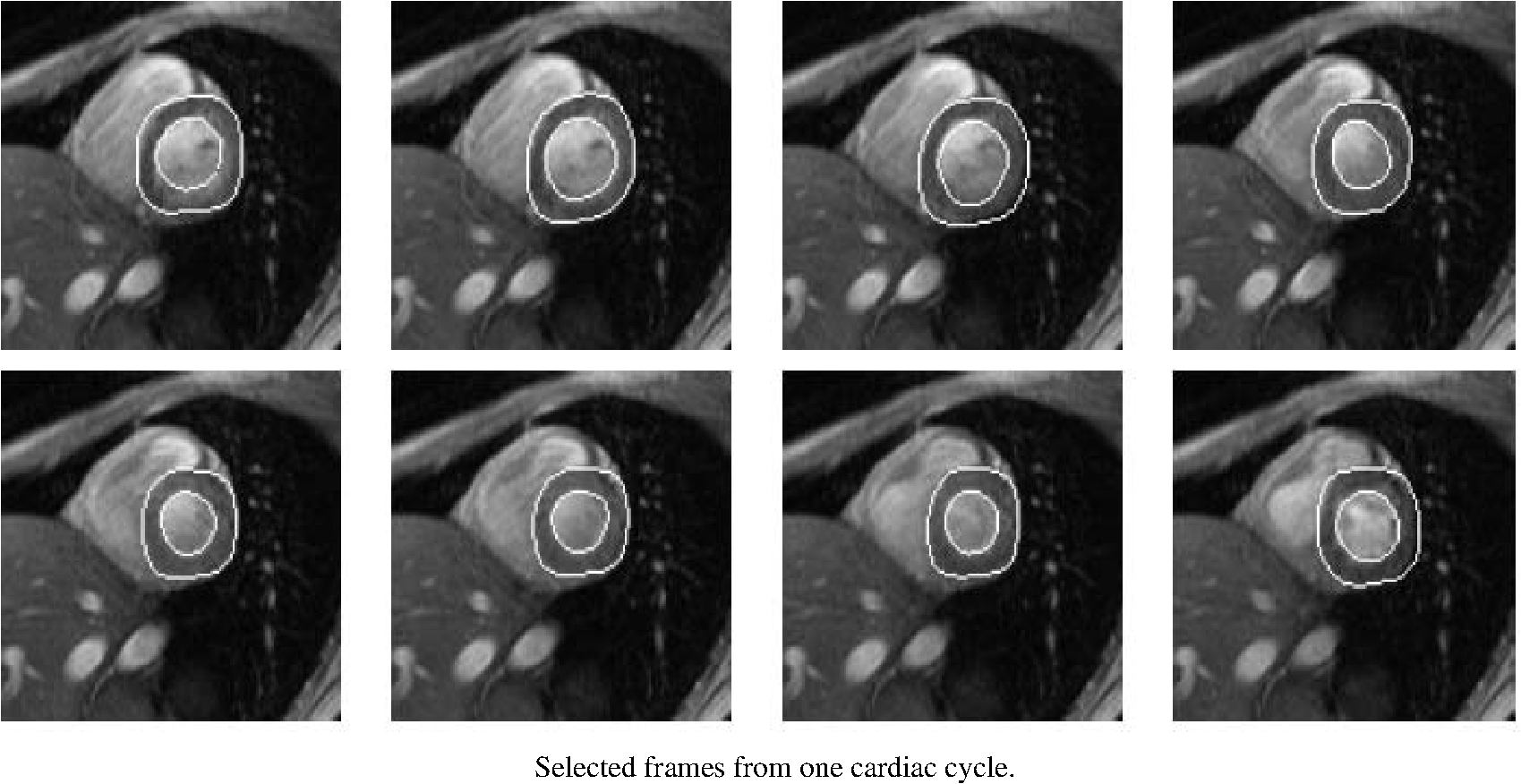 The interface is the zero level of (i.e., for all ). An evolution equation for then can be derived using as The contour evolution corresponds to an evolution of given by . The level-set based segmentation method has been extensively utilized in the image segmentation problems due to a variety of advantages: it is parameter free, implicit, can change the topology, and provides a direct way to estimate the geometric properties. In addition, a large amount of effort has been made for its performance improvement.27,29,31,47–50 In boundary-driven techniques, the gradient is used as a criterion to stop the curve. However, there are objects whose boundaries cannot be defined, such as smeared boundaries. Chan and Vese32 proposed a different model incorporating an implicit energy functional in boundaries with active contours and the level-set representation by modifying the Mumford-Shah functional, i.e., where a set of disjoint regions cover and on . is the number of image partitioning. Equation (14) is minimized in by setting to the mean of in . In the case of the two partitioning regions and , the Euler-Lagrange derivation of Eq. (14) is demonstrated by where is a Dirac delta function. Therefore, this energy minimization process depends on regional constants and the level-set function . is a balancing parameter between data fidelity and regularization.3.2.3.ClusteringClustering algorithms have been used to group image pixels of similar features in the image segmentation problems. The resulting pixel-cluster memberships provide a segmentation of the image. Clustering-based segmentation methods are considered to be an old yet robust technique.51–54 One of the widely used clustering techniques is the -means algorithm. This approach uses an objective function that expresses the performance of a representation for given clusters. If we represent the center of each image cluster by and the ’th element in cluster by , the objective function can be defined as Although this objective function produces clusters, it may not guarantee the convergence to the global minimum.55Another clustering-based segmentation method is the fuzzy c-means algorithm based on the -means and fuzzy set theory.56–58 The conventional fuzzy c-means method does not fully utilize the spatial information of the image. To cope with this limitation, an approach was developed to incorporate the spatial information into the objective function by indicating the strength of association between each pixel and a particular cluster (i.e., the probability that a pixel belongs to a specific cluster) in order to improve the segmentation results.59 In addition, the expectation-maximization (EM) algorithm using the Gaussian mixture model is one of the well-established clustering-based methods. The iterative algorithm uses the posterior probabilities and the maximum likelihood estimates of the means, covariances, and coefficients of the mixture model.60,61 Furthermore, the EM algorithm can be combined with various models such as the hidden Markov random field model in order to achieve accurate and robust segmentation results.62 However, clustering-based methods have a few weaknesses. The methods are sensitive to initialization, noise, and inhomogeneities of image intensities.63 3.3.Graph-Cuts TechniquesThe graph-cuts technique64,65 was originated from Greig's maximum a posteriori (MAP) estimation66 in order to find the maximum flow for binary images. An interactive graph-cuts technique can find a globally optimal segmentation of an image. The user selects some pixels called “seed points” as hard constraints inside the object to be segmented as well as some pixels belonging to the background. The objective function is typically defined by boundary and regional properties of the segments. Therefore the obtained segmentation provides the best balance of boundary and region properties satisfying the constraints.65 In the graph-cuts theory,65 an image is interpreted as a graph, where all pixels are connected to its neighbors. Graph node set and edge set connect nodes to form a graph . Terminals are two special nodes, known as the source (s) and sink (t), which are the start and end nodes of the flow in the graph, respectively. Also, there are two types of edges: n-links that connect neighboring pixels and t-links that connect pixels in image to terminal nodes. The cost or weight is assigned to each edge, . The costs of n-links are the penalties for discontinuities between the pixels, and the costs of t-links are the penalties for assigning the corresponding terminal to the pixel. Thus, the total cost of the n-links represents the cost of the boundary while the total cost of the t-links indicates the regional properties. A cut is a set of edges that separates the graph into regions connected to terminal nodes. The cost of a cut is defined by the sum of the costs of edges that belong to the cut, which is denoted by Then optimal segmentation results using the graph-cuts technique amount to finding the optimal solution for the cost of a cut, i.e., a minimal cost cut. An example of medical image segmentation using the graph-cuts techniques is illustrated in Fig. 4. Fig. 4LV segmentation examples for contrast cardiac CT images using the graph-cuts technique.67 The segmentation algorithm used here combines the EM-based region segmentation, the Dijkstra active contours using graph-cuts, and the shape information through a pattern matching strategy. The graph-cuts algorithm is used to cut the edges in the graph to form a closed-boundary contour between two different regions. (Reproduced from M. P. Jolly with permission of ©2006 Springer Science and Business Media.) 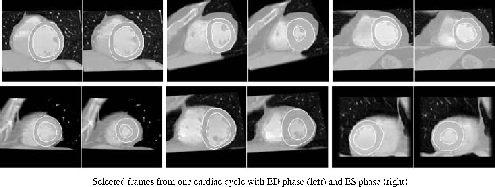 Several methods to find an optimal cost cut have been proposed such as minimizing the maximum cut between the segments68 and normalizing the cost of a cut.69 Boykov and Kolmogorov70 proposed a max-flow/min-cut algorithm and compared its efficiency with Goldberg-Tarjan's push-relabel71 and Ford-Fulkerson's augmenting paths.72 Based on the cut cost described above, the energy function can be formulated, consisting of the boundary term and the regional term. Let be the label for a given pixel , which can be either an object or the background. Let be a set of pixels and be a set of all pairs of neighboring elements. The energy function73 for graph-cuts can then be given by: where and where denotes the cost of n-link between two pixels and and denotes the cost of t-link at pixel . is a boundary term that imposes smoothness whereas is a region term that measures how well a label fits the data. is the interaction function between neighboring pixels and , and is a log-likelihood function at pixel .One limitation of the graph-cuts technique is that it is not fully automated, as it demands the initialization of seed points in the object and the background regions. 3.4.Model-Fitting TechniquesThe model-fitting segmentation attempts to match a predefined geometric shape to the locations of the extracted image features of an image. A two-step procedure is usually needed in the model-fitting segmentation: (1) generating the shape model from a training set and (2) performing the fitting of the model to a new image. The models contain the information about the shape and its variations. The main tasks in the model-fitting are the extraction of the features and generation of the best fitting model from the features. Given an accurate and appropriate model, the segmentation procedure becomes an optimization problem of finding the best model parameters for a given patient image. Human heart anatomy exhibits specific features and therefore the similar shape or intensity information about hearts can be utilized by means of a shape-prior knowledge. Prior knowledge can be used to compensate for common difficulties such as poor image contrast, noise, and missing boundaries. Integrating the prior knowledge using explicit shape representation into segmentation process has been a topic of interest for decades. For instance, global shape information with closed curves represented by Fourier descriptors was proposed where the Gaussian prior was assumed for Fourier coefficients.74,75 The shape model was built by learning the distribution of Fourier coefficients. In addition, active shape models (ASM) were used in a variety of segmentation tasks.18,76–78 In brief, key landmark points on each training image generate a statistical model of shape variation, and a statistical model of intensity is built by warping each example image to match the mean shape. Principal component analysis (PCA) is applied on the key landmark points where the sample distribution is assumed as a Gaussian distribution. Any sample within the distribution can be expressed as a mean shape with a linear combination of eigenvectors.79 Cootes et al.76,80,81 built statistical models by positioning control points across training images and developed the active appearance model (AAM).82 An example of image segmentation based on the AAM is illustrated in Fig. 5. The landmark points should be placed in a consistent way over a large database of training shapes in order to avoid incorrect parameterization.77 Also, if the size of a training set is small, the model cannot capture its variability and is unable to approximate data that are not included in the training set.78 Furthermore, a statistical model is incorporated in order to describe intersubject shape variabilities. For example, the dimension of the parametric contours was reduced by the use of PCA. By projecting the shape onto the shape parameters and enforcing limits, global shape constraints have been applied to ensure that the current shape remains similar to that in the training set.76 Wang and Staib84 extended the work of Cootes et al.76 using a Bayesian framework to adjust the weights between the statistical prior knowledge and the image information based on image quality and reliability of the training set. The B-splines based curve representation was applied to the classical active contours model.85–87 Fig. 5Segmentation results obtained by applying the AAM technique to an ultrasound image sequence over one heart beat period:83 (a) the initial 1-phase AAM model positioned, (b) the match after 5 AMM iterations, (c) the final match after 20 AAM iterations, and (d) the manual contours for comparison. The first row shows phase images 1, the second row shows phase images 2, and the third row shows phase images 3 from 16 image phases. (Reproduced from J. Bosch et al. with permission of ©2002 IEEE.) 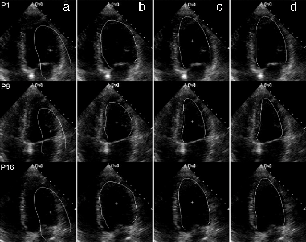 There have been several attempts to incorporate the prior knowledge of shape in the implicit shape representation. Leventon et al.88 incorporated the shape-prior information in the level-set framework with a set of previously segmented data using the signed distance function. A shape-prior model was also proposed to restrict the flow of the geodesic active contour, where the prior shape was derived by performing the PCA on a collection of the signed distance function of the training shape. A similar approach was proposed in Ref. 89 with an energy functional, including the information of the image gradient and the shape of interest in geometric active contours using the distance function to represent training distances. Another objective function for segmentation was proposed in Ref. 90 by applying the PCA to a collection of signed distance representations of the training data. Rousson and Paragios91 applied a shape constraint to the implicit representation using the level-set to formulate an energy functional, where an initial segmentation result can be corrected by the level-set shape prior model through PCA. They also considered a stochastic framework in constructing the shape model with two unknown variables: the shape image and the local degrees of shape deformations. In specific applications, 3-D heart modeling was explored in Ref. 19 and the four-chamber heart modeling was proposed in Refs. 1 and 92. Geometric constraint was also incorporated in the LV segmentation problem. The model-based approach in Ref. 93 has gained a lot of attention as a solution to the image segmentation problem with incomplete image information.94,95 Several other model-fitting methods have been investigated to date. The atlas-based segmentation was carried out based on the registration, where multiple atlases were registered to a target image by propagation of the atlas image labels with spatially varying decision fusion weight in CT scans.96 In addition, a deformable surface represented by a simplex mesh in the 3-D space used the time constraints in segmenting the SPECT cardiac image sequence in Ref. 2. Modeling the four-chamber heart was performed for 3-D cardiac CT segmentation,97 where the simplex meshes were used to provide a stable computation of curvature-based internal forces. Heart modeling was accomplished with a statistical shape model76 and labeling is performed on mesh points that correspond to special anatomical structures such as control points that integrate mesh models.1 The whole heart segmentation method, including four chambers, myocardium, and great vessels in CT images, was proposed in Ref. 98, where ASM and the generalized Hough transform for automatic model initialization were exploited. 4.Applications to Specific Imaging ModalitiesIn this section, several modalities for cardiac examinations are reviewed and techniques used for segmentation in each modality are presented. We summarize roles and characteristics of each modality with reference to the recent work,99 and describe the segmentation techniques used for each modality. 4.1.Ultrasound ImagingUS imaging is the most widely used technique in cardiology for evaluation of contractile cardiac function. It has several advantages, including good temporal resolution and relatively low cost. It can be used to assess tissue perfusion by myocardial contrast echocardiography.100 Additionally, it is well-suited for image-guided interventions due to its recent advances, allowing visualization of instruments as well as cardiac structures through the blood pool.101 However, US imaging suffers from low SNR (signal-to-noise ratio) and speckle noise,102 making the LV segmentation task challenging. Moreover, the acquisition is usually performed in 2-D102 and therefore depends on the orientation, leading to missing boundaries and low contrast between regions of interest.103 US imaging of the heart involves 2-D, 2-, 3-D, 3-, and Doppler echocardiography, each of which poses different challenges. In this review, we focus primarily on the segmentation of the 3-D and 3- data. A recent advance in this field of cardiac imaging is three-dimensional echocardiography (3-DE). This tool has been used only for research purposes in the past, but due to recent improvements in software algorithms and transducer technology, it is now used in clinical practice.104,105 2-D and 3-D echocardiography use different transducers. 3-DE is well-suited for LV mass, volumes, and EF104,105 because 2-D imaging can potentially provide biased measurements of EF.106 Numerous segmentation techniques have been proposed for US imaging. 3-D AAM was proposed,79,107 where its model was learned from the manual segmentation results and the information of the shape and image appearance of cardiac structures was included in a single model. The level-set or the active contour segmentation methods were also applied to the US segmentation.108–111 Level-set based method with specialized processing was adopted to extract highly curved volumes while ensuring smoothness of signals.108 Additionally, an algorithm based on deep neural networks and optimization was employed112 and a discriminative classifier, random forest, was used to delineate myocardium.113 For an in-depth review on the segmentation of US images, we refer the reader to Ref. 102. 4.2.Nuclear Imaging (SPECT and PET)Nuclear imaging has been an accepted clinical gold standard for the quantification of relative myocardial perfusion at stress and rest.114 It is also the mainstream imaging technique to estimate myocardial hypo-perfusion due to coronary stenosis. Gated myocardial perfusion SPECT115 is also widely used for the quantitative assessment of the LV function. LV regional wall motion and thickening by SPECT play an integral part to assess coronary artery disease and determine the extent and severity of functional abnormalities.116 Accurate segmentation of LV and quantification of the volume offer an objective means to determine the risk stratification and therapeutic strategy.117 However, delineation of the endocardial surface with nuclear imaging is challenging due to relatively low image resolution, extracardiac background activities, partial volume effect, count statistics, and reconstruction parameters.118 A few techniques have been developed for nuclear imaging segmentation. Germano et al.119 proposed LV segmentation method for SPECT, which is widely used in nuclear cardiology practice as illustrated in Fig. 6. In addition, wall motion and thickening were further investigated with the same technique.116 In brief, an asymmetric Gaussian was exploited to fit to each profile in each interval of a gated MPS volume, where a maximal count myocardial surface was determined. Other well-established methods for the quantitative analysis of nuclear myocardial perfusion imaging exist such as the Corridor4DM,120 the Emory Cardiac Toolbox,121 the University of Virginia quantification program,122 and the Yale quantification software.123 These automated software tools allow highly automatic definition of the LV contours and measure perfusion defect size, EF, EDV, and LV mass. Fig. 6The gated SPECT segmentation in Ref. 119, where the first row shows original myocardial perfusion SPECT (MPS) and the second row shows the segmented image of the first row.  In other developments, the level-set technique was employed for the segmentation of cardiac gated SPECT images124 and a geometric active contour-based SPECT segmentation technique was proposed.125 Slomka et al.126 and Declerck et al.127 proposed a template-based segmentation method using the registration-based approach. Additionally, the 4-D (3-) shape prior was adopted in Ref. 128 using implicit shape representation of the left myocardium in SPECT image segmentation. This study extended the shape modeling to the spatiotemporal domain by treating time as the fourth dimension and applied the 4-D PCA. Faber et al.129 employed an explicit edge detection method to estimate endocardial and epicardial boundaries using the structural information in gated SPECT perfusion images. The 3-D ASM segmentation algorithm was adopted in Refs. 118 and 130 for cardiac perfusion gated SPECT studies and the construction of geometrical shape and appearance models. Reutter et al.131 used a 3-D edge detection technique for the segmentation of respiratory-gated PET transmission images and Markov random fields were adopted for 3-D segmentation of cardiac PET images.132 4.2.1.Gated SPECT analysisIn gated cardiac imaging, a short and cyclic image sequence is generated, representing a single heartbeat that summarizes data acquired over cardiac cycles.133,134 Gated SPECT images can provide global and regional parameters of LV function as described in Sec. 2. Once LV is segmented,119,129,135 the endocardial and epicardial boundaries are utilized for the quantification of global and regional parameters. The LV cavity volume is determined by the volume of each voxel and number of voxels bound by the LV endocardium and valve plane.116,119,136 Measurements of EF including ES and ED from gated SPECT are validated in many studies, demonstrating good accuracy.8,119,136,137 However, the relatively low resolution of nuclear cardiac images can lead to an underestimation of the LV cavity size, especially when patients have small ventricles, therefore resulting in overestimation of the EF.138–140 Quantitative measurement of wall motion is obtained by displacements of the endocardium from ED to ES116,141,142 and WT quantification is measured by assessing the apparent intensity of the myocardium from ED to ES resulting from the partial volume effect.18,129,143–145 Despite the low resolution of gated MPS, partial volume effect is actually exploited to analyze motion and thickening, since changes in the image intensity are related to the thickening of the myocardium.116 4.3.Computer Tomography (CT)In cardiac CT, there are two imaging procedures: (1) coronary calcium scoring with noncontrast CT and (2) noninvasive imaging of coronary arteries with contrast-enhanced CT. Typically, noncontrast CT imaging exploits the natural density of tissues. As a result, various densities using different attenuation values such as air, calcium, fat, and soft tissues can be easily distinguished.146 Noncontrast CT imaging is a low-radiation exposure method within a single breath hold, determining the presence of coronary artery calcium.146 In comparison, contrast-enhanced CT is used for imaging of coronary arteries with contrast material such as a bolus or continuous infusion of a high concentration of iodinated contrast material.147 Furthermore, coronary CT angiography has been shown to be highly effective in detecting coronary stenosis.148 Especially in the recent rapid advances in CT technology, CT can provide detailed anatomical information of chambers, vessels, coronary arteries, and coronary calcium scoring. Coronary CT angiography can visualize not only the vessel lumen but also the vessel wall, allowing noninvasive assessment of the presence and the size of the noncalcified coronary plaque.149 Additionally, CT imaging provides functional as well as anatomical information, which can be used for quantitative assessment for systolic WT and regional wall motion.150,151 Various segmentation techniques have been proposed for cardiac CT applications. Funka-Lea et al.152 proposed a method to segment the entire heart using graph-cuts. Segmenting the entire heart was performed for clearer visualization of coronary vessels on the surface of the heart. They attempted to set up an initialization process to find seed regions automatically using a blowing balloon that measures the maximum heart volume and added an extra constraint with a blob energy term to the original graph-cuts formulation. Extracting the myocardium in 4-D cardiac MR and CT images was proposed in Ref. 67 using the graph-cuts as well as EM-based segmentation. Zheng et al.1 presented a segmentation method based on the marginal space learning by searching for the optimal smooth surface. Model-based techniques were also adopted for cardiac CT image segmentation using ASM with PCA.153 Methods for region growing154,155 and thresholding156,157 were also employed. An entirely different topic is the segmentation of coronary arteries from the CT angiography data, which is well covered by other reviews.158,159 4.4.MRICardiac MRI allows comprehensive cardiac assessment by several types of acquisitions that can be performed during one scanning session.9 It provides high-resolution visualization of cardiac chamber volumes, functions, and myocardial mass.160 Cardiac MRI has been established as the research gold standard for these measurements, with more and more clinical impact. Moreover, recently developed delayed enhancement imaging with gadolinium contrast has emerged as a highly sensitive and specific method for detecting myocardial necrosis. This allows improved evaluation of the myocardial infarction.161,162 Perfusion MRI imaging can also be performed for the diagnosis of ischemic heart disease. However, the perfusion MR imaging depends on a first-pass technique, which limits the conspicuity of perfusion defects.163,164 The advantages of MRI include exquisite soft-tissue contrast, high spatial resolution, low SNR, ability to characterize tissue with a variety of pulse sequences, and no ionizing radiation. Compared to PET or SPECT, the dependence of MR signal on regional hypoperfusion is minimal and does not prevent segmentation tasks. Some of the disadvantages are that cardiac MRI typically employs one breath-hold per slice with 5 to 15 slices per patient study, therefore necessitating multiple breath-holds for each patient dataset. Additionally, the images are of high-resolution in-plane but the resolution between slices is low (typically 8 to 10 mm). Also, multiple breath-hold acquisitions can cause errors in spatial alignment and result in artifacts of the 3-D heart image. These misalignments can be corrected by software registration techniques.165 Recently, full volume 3-D MRI acquisitions have been proposed.9 Cardiac MR tagging is an important reference technique to measure myocardial function, which allows quantification of local myocardial strain and strain rate.166,167 Tagged MR produces signals that can be used to track motion. Several techniques have been developed, including magnetization, saturation, spatial modulation of magnetization (SPAMM), delay alternating with nutation for tailored excitation (DANTE), and complementary SPAMM (CSPAMM). These techniques produce a visible pattern of magnetization saturation on the magnitude reconstructed image without any post-processing. However, quantifying myocardial motion requires exhaustive post-processing. In contrast, more advanced techniques such as Harmonic phase (HARP), displacement encoding with simulated echoes (DENSE), and strain encoding (SENC)167,168 compute motion directly from the signal and do not directly show tagging pattern. Simple post-processing is required for myocardial motion information. For more details, we refer readers to the recent review of cardiac tagged MRI.167 Numerous image segmentation techniques have been applied to MRI and are summarized below. Petitjean et al.169 presented a review of segmentation methods in short axis MR images. Paragios35 used the level-set technique using a geometric flow to segment endo- and epicardium of the LV. Two evolving contours were employed for the endo- and epicardium and the method combined the visual information with anatomical constraints to segment both regions of interest simultaneously. Paragios et al.35,170,171 applied the shape prior knowledge with the level-set representation to achieve robust and accurate results. Moreover, several constraints and prior knowledge have been incorporated in the level-set framework for efficiently segmenting regions of interest. For example, the velocity-constrained front propagation method was proposed by using the magnitude and direction of the phase contrast velocity as the constraints.172 Woo et al.173 proposed statistical distance between the shape of endo- and epicardium as a shape constraint using signed distance functions. Tsai et al.174 proposed a shape-based approach to curve evolution and Ciofolo et al.175 proposed a myocardium segmentation scheme for late-enhancement cardiac MR images by incorporating the shape prior with contour evolution. Zhu et al.176 applied a dynamic statistical shape model with the Bayesian method. Segmentation techniques using thresholding,177,178 region growing,179,180 and boundary detection181,182 were applied to MRI data. For instance, a local assessment of boundary detection method was proposed to improve the capture range and accuracy.183 Segmentation algorithm using optimal binary thresholding method and region growing was presented to delineate 3- cine MR images.184 In addition, learning frameworks were used to segment 2-D tagged cardiac MR images.185,186 4.5.Parameter Correlation between Imaging ModalitiesSeveral attempts have been made to compare and correlate the quantitative parameters obtained by different imaging modalities and different image segmentation approaches. Various reports in the literature indicate that cardiac MRI can provide accurate estimates of EF, LV volumes.187–191 and wall motion/thickening analysis.187–189 In addition, gated SPECT has been extensively validated against various two-dimensional imaging techniques, such as echocardiography,192 but there are only a limited number of studies comparing gated SPECT with other three-dimensional techniques such as cardiac MRI, which is considered the reference standard for assessing LV volumes.193–196 Visual interpretations of wall motion by observers on the two modalities have been compared along with LV volumes193–196 but quantitative comparison for assessment of regional wall motion/thickening has not been reported previously. Using echocardiographic sequences, values of LV volumes, EF, and regional endocardial shortening also correlate with MR. Cardiac MRI was used as a reference method for comparison with unenhanced and contrast-enhanced echocardiography.197,198 LV mass obtained by contrast enhanced color Doppler echocardiography has shown excellent agreement with those from MRI.199 The left and right ventricular EDV, ESV, stroke volume, EF, and myocardial mass obtained by dual-source CT also correlated well with those from MRI.200 5.Validation (Evaluation) of Segmentation ResultsAutomatic cardiac image segmentation results can be evaluated alone or by comparing it with a reference, possibly a different imaging modality, including the manual segmentation result or a ground truth. For stand-alone evaluation, one can exploit statistical properties of heart anatomy and/or observe the segmented images. For reference-based evaluation, both quantitative and qualitative comparisons can be performed. Quantitative comparison can be done by measuring various metrics such as the fractional energy difference, the Hausdorff distance, the average perpendicular distance, the dice metric, and the mean absolute distance110 between the segmented structures. The average perpendicular distance measures the distance from the automatically segmented contour to the corresponding manually drawn contour by experts, and averages of all contour points. For LV segmentation, the ED and the ES phases of all slices have been measured. The EF and the LV mass are also important clinical parameters to evaluate. Table 1 summarizes previous studies that dealt with cardiac segmentation validation with respect to different imaging modalities, imaging targets, the number of data sets, evaluation results, and comments. Table 1Cardiac image segmentation results with validation.
6.ConclusionsSeveral advanced segmentation techniques have been proposed in the image processing and computer vision communities for the cardiac image analysis. In this review, we have categorized them into four major classes: 1) the boundary-driven techniques, 2) the region-driven techniques, 3) the graph-cuts techniques, and 4) the model-fitting techniques. These techniques have been applied to segmentation of cardiac images acquired by different imaging modalities, providing high automation and accuracy in determining clinically significant parameters. These computational techniques aid clinicians in evaluation of the cardiac anatomy and function, and ultimately lead to improvements in patient care. However, cardiac image segmentation continues to remain a challenge due to the complex anatomy of the heart, limited spatial resolution, imaging characteristics, cardiac and respiratory motion, and variable pathology and anatomy. Therefore, improved segmentation techniques with enhanced reliability, reduced computation time, superior accuracy, and full automation will be needed for the future. ReferencesY. Zhenget al.,
“Four-chamber heart modeling and automatic segmentation for 3D cardiac CT volumes using marginal space learning and steerable features,”
IEEE Trans. Med. Imag., 27
(11), 1668
–1681
(2008). ITMID4 0278-0062 Google Scholar
J. MontagnatH. Delingette,
“4D deformable models with temporal constraints: application to 4D cardiac image segmentation,”
Med. Image Anal., 9
(1), 87
–100
(2005). http://dx.doi.org/10.1016/j.media.2004.06.025 1361-8415 Google Scholar
V. L. Rogeret al.,
“Heart disease and stroke statistics-2011 update: a report from the American Heart Association,”
Circulation, 123
(4), e18
–e209
(2011). http://dx.doi.org/10.1161/CIR.0b013e3182009701 CIRCAZ 0009-7322 Google Scholar
L. Bonneuxet al.,
“Estimating clinical morbidity due to ischemic heart disease and congestive heart failure: the future rise of heart failure,”
Am. J. Public Health, 84
(1), 20
–28
(1994). http://dx.doi.org/10.2105/AJPH.84.1.20 AJHEAA 0090-0036 Google Scholar
T. Makela,
“A review of cardiac image registration methods,”
IEEE Trans. Med. Imag., 21
(9), 1011
–1021
(2002). http://dx.doi.org/10.1109/TMI.2002.804441 ITMID4 0278-0062 Google Scholar
H. D. Whiteet al.,
“Left ventricular end-systolic volume as the major determinant of survival after recovery from myocardial infarction,”
Circulation, 76
(1), 44
–51
(1987). http://dx.doi.org/10.1161/01.CIR.76.1.44 CIRCAZ 0009-7322 Google Scholar
S. D. Solomonet al.,
“Influence of ejection fraction on cardiovascular outcomes in a broad spectrum of heart failure patients,”
Circulation, 112
(24), 3738
–3744
(2005). http://dx.doi.org/10.1161/CIRCULATIONAHA.105.561423 CIRCAZ 0009-7322 Google Scholar
G. Germanoet al.,
“A new algorithm for the quantitation of myocardial perfusion SPECT. Part I: technical principles and reproducibility,”
J. Nucl. Med., 41
(4), 712
–719
(2000). JNMEAQ 0161-5505 Google Scholar
C. PetitjeanJ. N. Dacher,
“A review of segmentation methods in short axis cardiac MR images,”
Med. Image Anal., 15
(2), 169
–184
(2010). 1361-8415 Google Scholar
G. Germanoet al.,
“Quantitation in gated perfusion SPECT imaging: the Cedars-Sinai approach,”
J. Nucl. Cardiol., 14
(4), 433
–454
(2007). http://dx.doi.org/10.1016/j.nuclcard.2007.06.008 JNCAE2 1071-3581 Google Scholar
L. Y. Hsuet al.,
“Quantitative myocardial infarction on delayed enhancement MRI. Part II: clinical application of an automated feature analysis and combined thresholding infarct sizing algorithm,”
J. Magn. Reson. Imag., 23
(3), 309
–314
(2006). 1053-1807 Google Scholar
M. D. Cerqueiraet al.,
“Standardized myocardial segmentation and nomenclature for tomographic imaging of the heart. A statement for healthcare professionals from the Cardiac Imaging Committee of the Council on Clinical Cardiology of the American Heart Association,”
Int. J. Cardiovasc. Imag., 18
(1), 539
–542
(2002). 1569-5794 Google Scholar
C. LorenzJ. von Berg,
“A comprehensive shape model of the heart,”
Med. Image Anal., 10
(4), 657
–670
(2006). http://dx.doi.org/10.1016/j.media.2006.03.004 1361-8415 Google Scholar
G. P. AurigemmaM. R. ZileW. H. Gaasch,
“Contractile behavior of the left ventricle in diastolic heart failure: with emphasis on regional systolic function,”
Circulation, 113
(2), 296
–304
(2006). http://dx.doi.org/10.1161/CIRCULATIONAHA.104.481465 CIRCAZ 0009-7322 Google Scholar
N. Beoharet al.,
“Quantitative assessment of regional left ventricular function with cardiac MRI: Three-dimensional centersurface method,”
Catheter. Cardio. Int., 69
(5), 721
–728
(2007). Google Scholar
E. R. Holmanet al.,
“Detection and quantification of dysfunctional myocardium by magnetic resonance imaging. A new three-dimensional method for quantitative wall-thickening analysis,”
Circulation, 95
(4), 924
–931
(1997). CIRCAZ 0009-7322 Google Scholar
R. J. van der Geestet al.,
“Quantitative analysis of cardiovascular MR images,”
Int. J. Cardiac Imag., 13
(3), 247
–258
(1997). http://dx.doi.org/10.1023/A:1005869509149 0167-9899 Google Scholar
A. Suinesiaputraet al.,
“Automated detection of regional wall motion abnormalities based on a statistical model applied to multislice short-axis cardiac MR images,”
IEEE Trans. Med. Imag., 28
(4), 595
–607
(2009). http://dx.doi.org/10.1109/TMI.2008.2008966 ITMID4 0278-0062 Google Scholar
A. F. FrangiW. J. NiessenM. A. Viergever,
“Three-dimensional modeling for functional analysis of cardiac images: a review,”
IEEE Trans. Med. Imag., 20
(1), 2
–5
(2001). http://dx.doi.org/10.1109/42.906421 ITMID4 0278-0062 Google Scholar
A. Abidovet al.,
“Transient ischemic dilation ratio of the left ventricle is a significant predictor of future cardiac events in patients with otherwise normal myocardial perfusion SPECT,”
J. Am. Coll. Cardiol., 42
(10), 1818
–1825
(2003). http://dx.doi.org/10.1016/j.jacc.2003.07.010 JACCDI 0735-1097 Google Scholar
M. KassA. WitkinD. Terzopoulos,
“Snakes: active contour models,”
Int. J. Comput. Vis., 1
(4), 321
–331
(1988). IJCVEQ 0920-5691 Google Scholar
M. KassA. WitkinD. Terzopoulos,
“Active contour models,”
Int. J. Comput. Vis., 1
(4), 321
–331
(1987). IJCVEQ 0920-5691 Google Scholar
C. XuJ. L. Prince,
“Snakes, shapes, and gradient vector flow,”
IEEE Trans. Image Process., 7
(3), 359
–369
(1998). IIPRE4 1057-7149 Google Scholar
L. D. Cohen,
“On active contour models and balloons,”
CVGIP: Image Understanding, 53
(2), 211
–218
(1991). http://dx.doi.org/10.1016/1049-9660(91)90028-N CIUNEJ 1049-9660 Google Scholar
I. MikicS. KrucinskiJ. D. Thomas,
“Segmentation and tracking in echocardiographic sequences: active contours guided by optical flow estimates,”
IEEE Trans. Med. Image, 17
(2), 274
–284
(1998). http://dx.doi.org/10.1109/42.700739 ITMID4 0278-0062 Google Scholar
V. CasellesR. KimmelG. Sapiro,
“Geodesic active contours,”
Int. J. Comput. Vis., 22
(1), 61
–79
(1997). http://dx.doi.org/10.1023/A:1007979827043 IJCVEQ 0920-5691 Google Scholar
S. Kichenassamyet al.,
“Gradient flows and geometric active contour models,”
in International Conference on Computer Vision (ICCV),
810
–815
(1995). http://dx.doi.org/10.1109/ICCV.1995.466855 Google Scholar
S. Kichenassamyet al.,
“Conformal curvature flows: from phase transitions to active vision,”
Arch. Ration. Mech. Anal., 134
(3), 275
–301
(1996). http://dx.doi.org/10.1007/BF00379537 AVRMAW 0003-9527 Google Scholar
A. J. Yezziet al.,
“A geometric snake model for segmentation of medical imagery,”
IEEE Trans. Med. Imag., 16
(2), 199
–209
(1997). http://dx.doi.org/10.1109/42.563665 ITMID4 0278-0062 Google Scholar
J. Sethian, Level Set Methods and Fast Marching Methods: Evolving Interfaces in Computational Geometry, Fluid Mechanics, Computer Vision, and Materials Science, Cambridge University Press, Cambridge
(1999). Google Scholar
V. Caselles,
“Geometric models for active contours,”
in Int. Conf. Image Process.,
C9
–C12
(1995). Google Scholar
T. ChanL. Vese,
“Active contours without edges,”
IEEE Trans. Image Process., 10
(2), 266
–277
(2001). http://dx.doi.org/10.1109/ICIP.1995.537567 IIPRE4 1057-7149 Google Scholar
N. ParagiosR. Deriche,
“Geodesic active regions and level set methods for motion estimation and tracking,”
Comput. Vision Image Understand., 97
(3), 259
–282
(2005). http://dx.doi.org/10.1016/j.cviu.2003.04.001 CVIUF4 1077-3142 Google Scholar
A. ChakrabortyL. H. StaibJ. S. Duncan,
“Deformable boundary finding influenced by region homogeneity,”
Comput. Vis. Pattern Recogn., 624
–627
(1994). http://dx.doi.org/10.1109/CVPR.1994.323790 Google Scholar
N. Paragios,
“A Variational Approach for the Segmentation of the Left Ventricle in Cardiac Image Analysis,”
Int. J. Comput. Vis., 50
(3), 345
–362
(2002). IJCVEQ 0920-5691 Google Scholar
D. MumfordJ. Shah,
“Boundary detection by minimizing functionals,”
in Int. Conf. Comput. Vision Pattern Recognit.,
22
–26
(1985). Google Scholar
C. V. AlvinoA. J. Yezzi,
“Fast Mumford-Shah segmentation using image scale space bases,”
Proc. SPIE, 6498 64980F
(2007). http://dx.doi.org/10.1117/12.715201 Google Scholar
T. BroxD. Cremers,
“On the statistical interpretation of the piecewise smooth Mumford-Shah functional,”
Scale Space Variation. Method. Comput. Vis., 4485 203
–213
(2007). Google Scholar
X. BressonP. VandergheynstJ. Thiran,
“A variational model for object segmentation using boundary information and shape prior driven by the Mumford-Shah functional,”
Int. J. Comput. Vis., 68
(2), 145
–162
(2006). http://dx.doi.org/10.1007/s11263-006-6658-x IJCVEQ 0920-5691 Google Scholar
Y. M. Chenet al.,
“Using prior shapes in geometric active contours in a variational framework,”
Int. J. Comput. Vis., 50
(3), 315
–328
(2002). http://dx.doi.org/10.1023/A:1020878408985 IJCVEQ 0920-5691 Google Scholar
D. CremersT. KohlbergerC. Schnorr,
“Nonlinear shape statistics in Mumford-Shah based segmentation,”
in Int. Conf. Eur. Conf. Comput. Vision,
516
–518
(2002). Google Scholar
A. TsaiA. J. YezziA. Willsky,
“Curve evolution implementation of the Mumford-Shah functional for image segmentation, denoising, interpolation, and magnification,”
IEEE Trans. Image Process., 10
(8), 1169
–1186
(2001). http://dx.doi.org/10.1109/83.935033 IIPRE4 1057-7149 Google Scholar
S. OsherJ. Sethian,
“Fronts propagating with curvature-dependent speed: algorithms based on Hamilton-Jacobi formulations,”
J. Comput. Phys., 79
(1), 12
–49
(1988). http://dx.doi.org/10.1016/0021-9991(88)90002-2 JCTPAH 0021-9991 Google Scholar
J. Sethian, Level Set Methods: Evolving Interfaces in Geometry, Fluid Mechanics, Computer Vision, and Materials Science, Cambridge University Press, Cambridge
(1996). Google Scholar
S. OsherR. Fedkiw, Level Set Methods and Dynamic Implicit Surfaces, Springer-Verlag , New York
(2002). Google Scholar
S. OsherN. Paragios, Geometric Level Set Methods in Imaging, Vision, and Graphics, Springer-Verlag, New York
(2003). Google Scholar
R. MalladiJ. SethianB. Vemuri,
“Shape modeling with front propagation: a level set approach,”
IEEE Trans. Pattern Anal. Mach. Intell., 17
(2), 158
–175
(1995). http://dx.doi.org/10.1109/34.368173 ITPIDJ 0162-8828 Google Scholar
N. ParagiosR. Deriche,
“Geodesic active contours and level sets for the detection and tracking of moving objects,”
IEEE Trans. Pattern Anal. Mach. Intell., 22
(3), 266
–280
(2000). http://dx.doi.org/10.1109/34.841758 ITPIDJ 0162-8828 Google Scholar
A. TsaiA. J. YezziA. S. Willsky,
“A curve evolution approach to smoothing and segmentation using the Mumford-Shah functional,”
in Int. Conf. Comput. Vision Pattern Recognit.,
119124
(2000). Google Scholar
E. SifakisC. GarciaG. Tziritas,
“Bayesian level sets for image segmentation,”
J. Vis. Comm.. Image Represent., 13
(1–2), 44
–64
(2002). http://dx.doi.org/10.1006/jvci.2001.0474 JVCRE7 1047-3203 Google Scholar
A. E. O. Boudraa,
“Automated detection of the left ventricular region in magnetic resonance images by Fuzzy C-Means model,”
Int. J. Cardiac Imag., 13
(4), 347
–355
(1997). http://dx.doi.org/10.1023/A:1005755819752 0167-9899 Google Scholar
C. W. ChenJ. LuoK. J. Parker,
“Image segmentation via adaptive K-mean clustering and knowledge-based morphological operations with biomedical applications,”
IEEE Trans. Image Process., 7
(12), 1673
–1683
(1998). http://dx.doi.org/10.1109/83.730379 IIPRE4 1057-7149 Google Scholar
M. C. Clarket al.,
“MRI segmentation using fuzzy clustering-techniques,”
IEEE Eng. Med. Biol. Magazine, 13
(5), 730
–742
(1994). http://dx.doi.org/10.1109/51.334636 IEMBDE 0739-5175 Google Scholar
H. P. Nget al.,
“Medical image segmentation using K-MEANS clustering and improved watershed algorithm,”
Southwest Symp. Image Anal. Interpretation, 241 61
–65
(2006). http://dx.doi.org/10.1109/SSIAI.2006.1633722 Google Scholar
G. B. ColemanH. C. Andrews,
“Image segmentation by clustering,”
Proc. IEEE, 67
(5), 773
–785
(1979). http://dx.doi.org/10.1109/PROC.1979.11327 IEEPAD 0018-9219 Google Scholar
J. C. BezdekL. O. HallL. P. Clarke,
“Review of MR image segmentation techniques using pattern recognition,”
Med. Phys., 20
(4), 1033
–1048
(1993). http://dx.doi.org/10.1118/1.597000 MPHYA6 0094-2405 Google Scholar
M. R. Rezaeeet al.,
“A multiresolution image segmentation technique based on pyramidalsegmentation and fuzzy clustering,”
IEEE Trans. Image Process., 9
(7), 1238
–1248
(2000). http://dx.doi.org/10.1109/83.847836 IIPRE4 1057-7149 Google Scholar
D. L. PhamJ. L. Prince,
“Adaptive fuzzy segmentation of magnetic resonance images,”
IEEE Trans. Med. Imag., 18
(9), 737
–752
(1999). http://dx.doi.org/10.1109/42.802752 ITMID4 0278-0062 Google Scholar
K. S. Chuanget al.,
“Fuzzy c-means clustering with spatial information for image segmentation,”
Comput. Med. Imag. Graph., 30
(1), 9
–15
(2006). http://dx.doi.org/10.1016/j.compmedimag.2005.10.001 CMIGEY 0895-6111 Google Scholar
C. Carsonet al.,
“Blobworld: Image segmentation using expectation-maximization and its application to image querying,”
IEEE Trans. Pattern Anal. Mach. Intell., 24
(8), 1026
–1038
(2002). http://dx.doi.org/10.1109/TPAMI.2002.1023800 ITPIDJ 0162-8828 Google Scholar
Z. LiangJ. MacFallD. Harrington,
“Parameter estimation and tissue segmentation from multispectral MR images,”
IEEE Trans. Med. Imag., 13
(3), 441
–449
(1994). http://dx.doi.org/10.1109/42.310875 ITMID4 0278-0062 Google Scholar
Y. ZhangM. BradyS. Smith,
“Segmentation of brain MR images through a hidden Markov random field model and the expectation-maximization algorithm,”
IEEE Trans. Med. Imag., 20
(1), 45
–57
(2001). http://dx.doi.org/10.1109/42.906424 ITMID4 0278-0062 Google Scholar
S. KrinidisV. Chatzis,
“A robust fuzzy local information C-Means clustering algorithm,”
IEEE Trans. Image Process., 19
(5), 1328
–1337
(2010). http://dx.doi.org/10.1109/TIP.2010.2040763 IIPRE4 1057-7149 Google Scholar
Y. BoykovO. VekslerR. Zabih,
“Fast approximate energy minimization via graph cuts,”
IEEE Trans. Pattern Anal. Mach. Intell., 23
(11), 1222
–1239
(2001). http://dx.doi.org/10.1109/34.969114 ITPIDJ 0162-8828 Google Scholar
Y. BoykovM. P. Jolly,
“Interactive graph cuts for optimal boundary & region segmentation of objects in N-D images,”
in Int. Conf. Comput. Vision,
105
–112
(2001). Google Scholar
D. GreigB. PorteousA. Seheult,
“Exact maximum a posteriori estimation for binary images,”
J. Roy. Statist. Soc. Ser. B (Methodological), 51
(2), 271
–279
(1989). JSTBAJ 0035-9246 Google Scholar
M. P. Jolly,
“Automatic segmentation of the left ventricle in cardiac MR and CT images,”
Int. J. Comput. Vis., 70
(2), 151
–163
(2006). http://dx.doi.org/10.1007/s11263-006-7936-3 IJCVEQ 0920-5691 Google Scholar
Z. WuR. Leahy,
“An optimal graph theoretic approach to data clustering: Theory and its application to image segmentation,”
IEEE Trans. Pattern Anal. Mach. Intell., 15
(11), 1101
–1113
(1993). http://dx.doi.org/10.1109/34.244673 ITPIDJ 0162-8828 Google Scholar
J. ShiJ. Malik,
“Normalized cuts and image segmentation,”
IEEE Trans. Pattern Anal. Mach. Intell., 22
(8), 888
–905
(2000). ITPIDJ 0162-8828 Google Scholar
Y. BoykovV. Kolmogorov,
“An experimental comparison of min-cut/max-flow algorithms for energy minimization in vision,”
IEEE Trans. Pattern Anal. Mach. Intell., 26
(9), 1124
–1137
(2004). http://dx.doi.org/10.1109/TPAMI.2004.60 ITPIDJ 0162-8828 Google Scholar
A. GoldbergR. Tarjan,
“A new approach to the maximum-flow problem,”
J. ACM, 35
(4), 921
–940
(1988). http://dx.doi.org/10.1145/48014.61051 JOACF6 0004-5411 Google Scholar
L. R. FordD. R. Fulkerson, Flows in Networks, Princeton University Press, Princeton, N. J.
(1962). Google Scholar
Y. BoykovG. Funka-Lea,
“Graph cuts and efficient nd image segmentation,”
Int. J. Comput. Vis., 70
(2), 109
–131
(2006). http://dx.doi.org/10.1007/s11263-006-7934-5 IJCVEQ 0920-5691 Google Scholar
K. DelibasisP. UndrillG. Cameron,
“Designing Fourier descriptor-based geometric models for object interpretation in medical images using genetic algorithms,”
Comput. Vision Image Understand., 66
(3), 286
–300
(1997). http://dx.doi.org/10.1006/cviu.1996.0505 CVIUF4 1077-3142 Google Scholar
L. H. StaibJ. S. Duncan,
“Boundary finding with parametrically deformable models,”
IEEE Trans. Pattern Anal. Mach. Intell., 14
(11), 1061
–1075
(1992). http://dx.doi.org/10.1109/34.166621 ITPIDJ 0162-8828 Google Scholar
T. Cooteset al.,
“Active shape models-their training and application,”
Comput. Vis. Image Understand., 61
(1), 38
–59
(1995). http://dx.doi.org/10.1006/cviu.1995.1004 CVIUF4 1077-3142 Google Scholar
H. C. van Assenet al.,
“SPASM: a 3D-ASM for segmentation of sparse and arbitrarily oriented cardiac MRI data,”
Med. Image Anal., 10
(2), 286
–303
(2006). http://dx.doi.org/10.1016/j.media.2005.12.001 1361-8415 Google Scholar
H. Zhanget al.,
“4-D cardiac MR image analysis: left and right ventricular morphology and function,”
IEEE Trans. Med. Imag., 29
(2), 350
–364
(2010). http://dx.doi.org/10.1109/TMI.2009.2036843 ITMID4 0278-0062 Google Scholar
S. C. Mitchellet al.,
“3-D active appearance models: segmentation of cardiac MR and ultrasound images,”
IEEE Trans. Med. Imag., 21
(9), 1167
–1178
(2002). http://dx.doi.org/10.1109/TMI.2002.804425 ITMID4 0278-0062 Google Scholar
T. CootesA. HillC. TaylorJ. Haslam,
“The use of active shape models for locating structures in medical images,”
Image Vis. Comput., 12
(6), 355
–366
(1994). http://dx.doi.org/10.1016/0262-8856(94)90060-4 IVCODK 0262-8856 Google Scholar
T. CootesC. Taylor,
“Active shape models-smart snakes,”
in British Machine Vision Conference,,
266
–275
(1992). Google Scholar
T. CootesG. EdwardsC. Taylor,
“Active appearance models,”
IEEE Trans. Pattern Anal. Mach. Intell., 23
(6), 681
–685
(2001). http://dx.doi.org/10.1109/34.927467 ITPIDJ 0162-8828 Google Scholar
J. Boschet al.,
“Automatic segmentation of echocardiographic sequences by active appearance motion models,”
IEEE Trans. Med. Imag., 21
(11), 1374
–1383
(2002). http://dx.doi.org/10.1109/TMI.2002.806427 ITMID4 0278-0062 Google Scholar
Y. WangL. Staib,
“Boundary Finding with Correspondence Using Statistical Shape Models,”
in Int. Conf. Comput. Vision Pattern Recognit.,,
338
–345
(1998). Google Scholar
D. CremersT. KohlbergerC. Schnorr,
“Shape statistics in kernel space for variational image segmentation,”
Pattern Recogn., 36
(9), 1929
–1943
(2003). http://dx.doi.org/10.1016/S0031-3203(03)00056-6 PTNRA8 0031-3203 Google Scholar
D. CremersC. SchnorrJ. Weickert,
“Diffusion-snakes: Combining statistical shape knowledge and image information in a variational framework,”
in IEEE Workshop on Variational and Level Set Methods in Computer Vision,
137
–144
(2001). Google Scholar
D. Cremerset al.,
“Diffusion snakes: Introducing statistical shape knowledge into the Mumford-Shah functional,”
Int. J. Comput. Vis., 50
(3), 295
–313
(2002). http://dx.doi.org/10.1023/A:1020826424915 IJCVEQ 0920-5691 Google Scholar
M. LeventonW. GrimsonO. Faugeras,
“Statistical shape influence in geodesic active contours,”
Comput. Vision Pattern Recogn., 1 316
–322
(2000). http://dx.doi.org/10.1109/SSBI.2002.1233989 Google Scholar
Y. M. Chenet al.,
“On the incorporation of shape priors into geometric active contours,”
in IEEE Workshop on Variational and Level Set Methods in Computer Vision,
145
–152
(2001). Google Scholar
A. Tsaiet al.,
“Model-based curve evolution technique for image segmentation,”
Computer Vis. Pattern Recogn., 1186 463
–468
(2001). http://dx.doi.org/10.1109/CVPR.2001.990511 Google Scholar
M. RoussonN. Paragios,
“Shape priors for level set representations,”
in European Conf. on Computer Vision,
78
–92
(2002). Google Scholar
Y. Zhenget al.,
“Fast automatic heart chamber segmentation from 3D CT data using marginal space learning and steerable features,”
in Int. Conf. on Computer Vision,
762
–769
(2007). Google Scholar
P. J. Slomkaet al.,
“Three-dimensional demarcation of perfusion zones corresponding to specific coronary arteries: application for automated interpretation of myocardial SPECT,”
J. Nucl. Med., 36
(11), 2120
–2126
(1995). JNMEAQ 0161-5505 Google Scholar
D. CremersS. OsherS. Soatto,
“Kernel density estimation and intrinsic alignment for shape priors in level set segmentation,”
Int. J. Comput. Vis., 69
(3), 335
–351
(2006). http://dx.doi.org/10.1007/s11263-006-7533-5 IJCVEQ 0920-5691 Google Scholar
M. RoussonN. ParagiosR. Deriche,
“Implicit active shape models for 3D segmentation in MR imaging,”
Med. Image Comput. Comput. Assist. Interv., 3216 209
–216
(2004). Google Scholar
I. Isgumet al.,
“Multi-atlas-based segmentation with local decision fusion-application to cardiac and aortic segmentation in CT scans,”
IEEE Trans. Med. Imag., 28
(7), 1000
–1010
(2009). http://dx.doi.org/10.1109/TMI.2008.2011480 ITMID4 0278-0062 Google Scholar
H. Delingette,
“General object reconstruction based on simplex meshes,”
Int. J. Comput. Vis., 32
(2), 111
–146
(1999). http://dx.doi.org/10.1023/A:1008157432188 IJCVEQ 0920-5691 Google Scholar
O. Ecabertet al.,
“Automatic model-based segmentation of the heart in CT images,”
IEEE Trans. Med. Imag., 27
(9), 1189
–1201
(2008). http://dx.doi.org/10.1109/TMI.2008.918330 ITMID4 0278-0062 Google Scholar
D. S. Bermanet al.,
“Comparative roles of cardiac CT and nuclear cardiology in assessment of the patient with suspected coronary artery disease,”
J. Invasive Cardiol., 21
(7), 352
–358
(2009). 1042-3931 Google Scholar
S. M. Bieriget al.,
“Comparison of myocardial contrast echocardiography derived myocardial perfusion reserve with invasive determination of coronary flow reserve,”
Eur. J. Echocardiogr., 10
(2), 250
–255
(2009). 1525-2167 Google Scholar
M. G. Linguraruet al.,
“Atrial septal defect tracking in 3D cardiac ultrasound,”
Med. Image Comput. Comput. Assist. Interv., 9
(Pt 1), 596
–603
(2006). Google Scholar
J. A. NobleD. Boukerroui,
“Ultrasound image segmentation: a survey,”
IEEE Trans. Med. Imag., 25
(8), 987
–1010
(2006). http://dx.doi.org/10.1109/TMI.2006.877092 ITMID4 0278-0062 Google Scholar
S. L. Bridalet al.,
“Milestones on the road to higher resolution, quantitative, and functional ultrasonic imaging,”
Proc. IEEE, 91
(10), 1543
–1561
(2003). http://dx.doi.org/10.1109/JPROC.2003.817879 IEEPAD 0018-9219 Google Scholar
A. BhanS. KapetanakisM. J. Monaghan,
“Three-dimensional echocardiography,”
Heart, 96
(2), 153
–163
(2010). Google Scholar
A. E. Weyman,
“The year in echocardiography,”
J .Am. Coll. Cardiol., 53
(17), 1558
–1567
(2010). JACCDI 0735-1097 Google Scholar
J. L. Hareet al.,
“Feasibility and clinical decision-making with 3D echocardiography in routine practice,”
Heart, 94
(4), 440
–445
(2008). Google Scholar
M. Maet al.,
“Model driven quantification of left ventricular function from sparse single-beat 3D echocardiography,”
Med. Image Anal., 14
(4), 582
–593
(2010). http://dx.doi.org/10.1016/j.media.2010.04.004 1361-8415 Google Scholar
E. D. Angeliniet al.,
“Segmentation of real-time three-dimensional ultrasound for quantification of ventricular function: a clinical study on right and left ventricles,”
Ultrasound Med. Biol., 31
(9), 1143
–1158
(2005). http://dx.doi.org/10.1016/j.ultrasmedbio.2005.03.016 USMBA3 0301-5629 Google Scholar
Y. YueH. D. Tagare,
“Evaluation of a level set segmentation method for cardiac ultrasound images—art. no. 69200E,”
Proc. SPIE, 6920 69200E
(2008). http://dx.doi.org/10.1016/j.ultrasmedbio.2005.03.016 Google Scholar
Y. Yueet al.,
“Evaluation of a cardiac ultrasound segmentation algorithm using a phantom,”
Med. Image Comput. Comput. Assis. Interv., 11
(Pt 1), 101
–109
(2008). Google Scholar
Y. ZhuX. PapademetrisA. J. SinusasJ. S. Duncan,
“A coupled deformable model for tracking myocardial borders from real-time echocardiography using an incompressibility constraint,”
Med. Image Anal., 14
(3), 429
–448
(2010). http://dx.doi.org/10.1016/j.media.2010.02.005 1361-8415 Google Scholar
G. CarneiroJ. NascimentoA. Freitas,
“Robust left ventricle segmentation from ultrasound data using deep neural networks and efficient search methods,”
in Int. Symp. on Biomedical Imaging,
1085
–1088
(2010). Google Scholar
V. Lempitskyet al.,
“Random forest classification for automatic delineation of myocardium in real-time 3D echocardiography,”
in Int. Conf. on Functional Imaging and Modeling of the Heart,
447
–456
(2009). Google Scholar
P. J. Slomkaet al.,
“Advances in technical aspects of myocardial perfusion SPECT imaging,”
J. Nucl. Cardiol., 16
(2), 255
–276
(2009). http://dx.doi.org/10.1007/s12350-009-9052-6 JNCAE2 1071-3581 Google Scholar
A. K. PaulH. A. Nabi,
“Gated myocardial perfusion SPECT: basic principles, technical aspects, and clinical applications,”
J. Nucl. Med. Technol., 32
(4), 179
–87
(2004). JNMTB4 0091-4916 Google Scholar
G. GermanoJ. ErelH. Lewinet al.,
“Automatic quantitation of regional myocardial wall motion and thickening from gated technetium-99 m sestamibi myocardial perfusion single-photon emission computed tomography,”
J. Am. Coll. Cardiol., 30
(5), 1360
–1367
(1997). http://dx.doi.org/10.1016/S0735-1097(97)00276-3 JACCDI 0735-1097 Google Scholar
T. Schepiset al.,
“Comparison of 64-slice CT with gated SPECT for evaluation of left ventricular function,”
J. Nucl. Med., 47
(8), 1288
–1294
(2006). JNMEAQ 0161-5505 Google Scholar
C. Tobon-Gomezet al.,
“Automatic construction of 3D-ASM intensity models by simulating image acquisition: application to myocardial gated SPECT studies,”
IEEE Trans. Med. Imag., 27
(11), 1655
–1667
(2008). http://dx.doi.org/10.1109/TMI.2008.2004819 ITMID4 0278-0062 Google Scholar
G. Germanoet al.,
“Automatic quantification of ejection fraction from gated myocardial perfusion SPECT,”
J. Nucl. Med., 36
(11), 2138
–2147
(1995). JNMEAQ 0161-5505 Google Scholar
E. P. Ficaroet al.,
“Corridor4DM: the Michigan method for quantitative nuclear cardiology,”
J. Nucl. Cardiol., 14
(4), 455
–465
(2007). http://dx.doi.org/10.1016/j.nuclcard.2007.06.006 JNCAE2 1071-3581 Google Scholar
E. V. Garciaet al.,
“The increasing role of quantification in clinical nuclear cardiology: the Emory approach,”
J. Nucl. Cardiol., 14
(4), 420
–432
(2007). http://dx.doi.org/10.1016/j.nuclcard.2007.06.009 JNCAE2 1071-3581 Google Scholar
D. D. WatsonW. H. Smith,
“The role of quantitation in clinical nuclear cardiology: the University of Virginia approach,”
J. Nucl. Cardiol., 14
(4), 466
–482
(2007). http://dx.doi.org/10.1016/j.nuclcard.2007.06.007 JNCAE2 1071-3581 Google Scholar
Y. H. Liu,
“Quantification of nuclear cardiac images: the Yale approach,”
J. Nucl. Cardiol., 14
(4), 483
–491
(2007). http://dx.doi.org/10.1016/j.nuclcard.2007.06.005 JNCAE2 1071-3581 Google Scholar
E. Debreuveet al.,
“Space-time segmentation using level set active contours applied to myocardial gated SPECT,”
IEEE Trans. Med. Imag., 20
(7), 643
–659
(2001). http://dx.doi.org/10.1109/42.932748 ITMID4 0278-0062 Google Scholar
R. YangM. MirmehdiaD. Hallb,
“A charged contour model for cardiac SPECT segmentation,”
171
–175
(2006). Google Scholar
P. J. Slomkaet al.,
“Automated alignment and sizing of myocardial stress and rest scans to three-dimensional normal templates using an image registration algorithm,”
J. Nucl. Med., 36
(6), 1115
–1122
(1995). JNMEAQ 0161-5505 Google Scholar
J. Declercket al.,
“Automatic registration and alignment on a template of cardiac stress and rest reoriented SPECT images,”
IEEE Trans. Med. Imag., 16
(6), 727
–737
(1997). http://dx.doi.org/10.1109/42.650870 ITMID4 0278-0062 Google Scholar
T. Kohlbergeret al.,
“4D shape priors for a level set segmentation of the left myocardium in SPECT sequences,”
Int. Conf. on Med. Image Comput. Comput. Assis. Interv., 9
(Pt 1), 92
–100
(2006). Google Scholar
T. L. Faberet al.,
“Left ventricular function and perfusion from gated SPECT perfusion images: an integrated method,”
J. Nucl. Med., 40
(4), 650
–659
(1999). JNMEAQ 0161-5505 Google Scholar
S. Ordaset al.,
“A statistical model-based approach for the automatic quantitative analysis of perfusion gated SPECT studies,”
Proc. SPIE, 5746 560
–570
(2005). http://dx.doi.org/10.1117/12.595897 Google Scholar
B. W. ReutterG. J. KleinR. H. Huesman,
“Automated 3-D segmentation of respiratory-gated PET transmission images,”
IEEE Trans. Nucl. Sci., 44
(6), 2473
–2476
(1997). http://dx.doi.org/10.1109/23.656454 IETNAE 0018-9499 Google Scholar
A. JuslinJ. Tohka,
“Unsupervised segmentation of cardiac PET transmission images for automatic heart volume extraction,”
in Conf. Proc. IEEE Engineering in Medicine and Biology Society,
1979
–1982
(2006). Google Scholar
M. P. SandlerR. E. ColemanJ. A. Patton, Diagnostic Nuclear Medicine, Lippincott Williams & Wilkins, Philadelphia
(2003). Google Scholar
M. N. WernickJ. N. Aarsvold,
“Emission Tomography: The Fundamentals of PET and SPECT,”
Academic Press, San Diego
(2004). Google Scholar
E. P. FicaroJ. R. Corbett,
“Advances in quantitative perfusion SPECT imaging,”
J. Nucl. Cardiol., 11
(1), 62
–70
(2004). http://dx.doi.org/10.1016/j.nuclcard.2003.10.007 JNCAE2 1071-3581 Google Scholar
G. Germanoet al.,
“Quantitative LVEF and qualitative regional function from gated thallium-201 perfusion SPECT,”
J. Nucl. Med., 38
(5), 749
–754
(1997). JNMEAQ 0161-5505 Google Scholar
T. L. Faberet al.,
“Evaluation of left ventricular endocardial volumes and ejection fractions computed from gated perfusion SPECT with magnetic resonance imaging: comparison of two methods,”
J. Nucl. Cardiol., 8
(6), 645
–651
(2001). http://dx.doi.org/10.1067/mnc.2001.117173 JNCAE2 1071-3581 Google Scholar
P. V. Fordet al.,
“Overestimation of the LVEF by quantitative gated SPECT in simulated left ventricles,”
J. Nucl. Med., 42
(3), 454
–459
(2001). JNMEAQ 0161-5505 Google Scholar
A. S. HambyeA. VervaetA. Dobbeleir,
“Variability of left ventricular ejection fraction and volumes with quantitative gated SPECT: influence of algorithm, pixel size and reconstruction parameters in small and normal-sized hearts,”
Eur. J. Nucl. Med. Mol. Imag., 31
(12), 1606
–1613
(2004). http://dx.doi.org/10.1007/s00259-004-1601-2 1619-7070 Google Scholar
K. Nakajimaet al.,
“Gated SPET quantification of small hearts: mathematical simulation and clinical application,”
Eur. J. Nucl. Med., 27
(9), 1372
–1379
(2000). http://dx.doi.org/10.1007/s002590000299 EJNMD9 0340-6997 Google Scholar
T. L. Faberet al.,
“A model-based four-dimensional left ventricular surface detector,”
IEEE Trans. Med. Imag., 10
(3), 321
–329
(1991). http://dx.doi.org/10.1109/42.97581 ITMID4 0278-0062 Google Scholar
K. T. YangH. D. Chen,
“Evaluation of global and regional left ventricular function using technetium-99m sestamibi ECG-gated single-photon emission tomography,”
Eur. J. Nucl. Med., 25
(5), 515
–521
(1998). http://dx.doi.org/10.1007/s002590050252 EJNMD9 0340-6997 Google Scholar
T. Shariret al.,
“Quantitative analysis of regional motion and thickening by gated myocardial perfusion SPECT: normal heterogeneity and criteria for abnormality,”
J. Nucl. Med., 42
(11), 1630
–1638
(2001). JNMEAQ 0161-5505 Google Scholar
K. Fukuchiet al.,
“Quantification of systolic count increase in technetium-99m-MIBI gated myocardial SPECT,”
J. Nucl. Med., 38
(7), 1067
–1073
(1997). JNMEAQ 0161-5505 Google Scholar
J. C. Stollfusset al.,
“Regional myocardial wall thickening and global ejection fraction in patients with low angiographic left ventricular ejection fraction assessed by visual and quantitative resting ECG-gated 99mTc-tetrofosmin single-photon emission tomography and magnetic resonance imaging,”
Eur. J. Nucl. Med., 25
(5), 522
–530
(1998). http://dx.doi.org/10.1007/s002590050253 EJNMD9 0340-6997 Google Scholar
D. Deyet al., Comprehensive Non-contrast CT Imaging of the Vulnerable Patient Asymptomatic Atherosclerosis, Humana Press, New York
(2010). Google Scholar
U. Schoepf,
“CT of the Heart: Principles and Applications,”
Humana Press Inc.(2005). Google Scholar
W. B. Meijboomet al.,
“Diagnostic accuracy of 64-slice computed tomography coronary angiography: a prospective, multicenter, multivendor study,”
J. Am. Coll. Cardiol., 52
(25), 2135
–2144
(2008). http://dx.doi.org/10.1016/j.jacc.2008.08.058 JACCDI 0735-1097 Google Scholar
D. Deyet al.,
“Automated three-dimensional quantification of noncalcified coronary plaque from coronary CT angiography: comparison with intravascular US,”
Radiology, 257
(2), 516
–522
(2010). http://dx.doi.org/10.1148/radiol.10100681 RADLAX 0033-8419 Google Scholar
T. S. Kristensenet al.,
“Quantitative assessment of left ventricular systolic wall thickening using multidetector computed tomography,”
Eur. J. Radiol., 72
(1), 92
–97
(2009). http://dx.doi.org/10.1016/j.ejrad.2008.06.028 EJRADR 0720-048X Google Scholar
E. D. Nicolet al.,
“64-Channel cardiac computed tomography: intraobserver and interobserver variability, part 2: global and regional ventricular function, mass, and first pass perfusion,”
J. Comput. Assist. Tomogr., 33
(2), 169
–174
(2009). JCATD5 0363-8715 Google Scholar
G. Funka-Leaet al.,
“Automatic heart isolation for CT coronary visualization using graph-cuts,”
in Int. Symp. on Biomedical Imaging,
614
–617
(2006). Google Scholar
O. EcabertJ. PetersJ. Weese,
“Modeling shape variability for full heart segmentation in cardiac computed-tomography images,”
Proc. SPIE, 6144 61443R
(2006). http://dx.doi.org/10.1117/12.652105 Google Scholar
D. Deyet al.,
“Automated quantitation of pericardiac fat from noncontrast CT,”
Invest. Radiol., 43
(2), 145
–153
(2008). http://dx.doi.org/10.1097/RLI.0b013e31815a054a INVRAV 0020-9996 Google Scholar
G. Muhlenbruchet al.,
“Global left ventricular function in cardiac Evaluation CT. of an automated 3D region-growing segmentation algorithm,”
Eur. Radiol., 16
(5), 1117
–1123
(2006). http://dx.doi.org/10.1007/s00330-005-0079-z EURAE3 1432-1084 Google Scholar
K. U. Juergenset al.,
“Automated threshold-based 3D segmentation versus short-axis planimetry for assessment of global left ventricular function with dual-source MDCT,”
Am. J. Roentgenol., 190
(2), 308
–314
(2008). http://dx.doi.org/10.2214/AJR.07.2283 AJROAM 0092-5381 Google Scholar
R. Yalamanchiliet al.,
“Knowledge-based quantification of pericardial fat in non-contrast CT data,”
Proc. SPIE, 7623 76231X
(2010). http://dx.doi.org/10.1117/12.843867 Google Scholar
C. KirbasF. Quek,
“A review of vessel extraction techniques and algorithms,”
ACM Comput. Surv., 36
(2), 81
–121
(2004). http://dx.doi.org/10.1145/1031120 ACSUEY 0360-0300 Google Scholar
D. Lesageet al.,
“A review of 3D vessel lumen segmentation techniques: models, features and extraction schemes,”
Med. Image Anal., 13
(6), 819
–845
(2009). http://dx.doi.org/10.1016/j.media.2009.07.011 1361-8415 Google Scholar
K. Alfakihet al.,
“Assessment of ventricular function and mass by cardiac magnetic resonance imaging,”
Eur. Radiol., 14
(10), 1813
–1822
(2004). http://dx.doi.org/10.1007/s00330-004-2387-0 EURAE3 1432-1084 Google Scholar
R. J. Kimet al.,
“Relationship of MRI delayed contrast enhancement to irreversible injury, infarct age, and contractile function,”
Circulation, 100
(19), 1992
–2002
(1999). CIRCAZ 0009-7322 Google Scholar
P. Hunoldet al.,
“Myocardial late enhancement in contrast-enhanced cardiac MRI: distinction between infarction scar and non-infarction-related disease,”
AJR Am. J. Roentgenol., 184
(5), 1420
–1426
(2005). AAJRDX 0361-803X Google Scholar
D. S. Bermanet al.,
“Roles of nuclear cardiology, cardiac computed tomography, and cardiac magnetic resonance: assessment of patients with suspected coronary artery disease,”
J. Nucl. Med., 47
(1), 74
–82
(2006). JNMEAQ 0161-5505 Google Scholar
M. IshidaS. KatoH. Sakuma,
“Cardiac MRI in ischemic heart disease,”
Circ. J., 73
(9), 1577
–1588
(2009). http://dx.doi.org/10.1253/circj.CJ-09-0524 1346-9843 Google Scholar
P. J. Slomkaet al.,
“Patient motion correction for multiplanar, multi-breath-hold cardiac cine MR imaging,”
J. Magn. Reson. Imag., 25
(5), 965
–973
(2007). http://dx.doi.org/10.1002/(ISSN)1522-2586 1053-1807 Google Scholar
E. A. Zerhouniet al.,
“Human heart: tagging with MR imaging: a method for noninvasive assessment of myocardial motion,”
Radiology, 169
(1), 59
–63
(1988). RADLAX 0033-8419 Google Scholar
S. H. Ibrahim el,
“Myocardial tagging by Cardiovascular Magnetic Resonance: evolution of techniques--pulse sequences, analysis algorithms, and applications,”
J. Cardiovasc. Magn. Reson., 13
(36), 36
–75
(2011). http://dx.doi.org/10.1186/1532-429X-13-36 Google Scholar
S. H. Ibrahim elet al.,
“Real-time MR imaging of myocardial regional function using strain-encoding (SENC) with tissue through-plane motion tracking,”
J. Magn. Reson. Imag., 26
(6), 1461
–1470
(2007). Google Scholar
C. PetitjeanJ. N. Dacher,
“A review of segmentation methods in short axis cardiac MR images,”
Med. Image Anal., 15
(2), 169
–184
(2011). http://dx.doi.org/10.1016/j.media.2010.12.004 1361-8415 Google Scholar
N. Paragios,
“Variational methods and partial differential equations in cardiac image analysis,”
in Int. Symp. on Biomedical Imaging,
17
–20
(2004). Google Scholar
N. Paragios,
“A level set approach for shape-driven segmentation and tracking of the left ventricle,”
IEEE Trans. Med. Imag., 22
(6), 773
–776
(2003). http://dx.doi.org/10.1109/TMI.2003.814785 ITMID4 0278-0062 Google Scholar
A. L. N. WongH. F. LiuP. C. Shi,
“Segmentation of myocardium using velocity field constrained front propagation,”
in IEEE Workshop on Applications of Computer Vision,
84
–89
(2002). Google Scholar
J. Wooet al.,
“Curve evolution with a dual shape similarity and its application to segmentation of left ventricle,”
Proc. SPIE, 7529 72593T
(2009). http://dx.doi.org/10.1117/12.814142 Google Scholar
A. Tsaiet al.,
“A shape-based approach to the segmentation of medical imagery using level sets,”
IEEE Trans. Med. Imag., 22
(2), 137
–154
(2003). http://dx.doi.org/10.1109/TMI.2002.808355 ITMID4 0278-0062 Google Scholar
C. Ciofoloet al.,
“Automatic myocardium segmentation in late-enhancement MRI,”
in Int. Symp. on Biomedical Imaging,
225
–228
(2008). Google Scholar
Y. Zhuet al.,
“Segmentation of the left ventricle from cardiac MR images using a subject-specific dynamical model,”
IEEE Trans. Med. Imag., 29
(3), 669
–687
(2009). ITMID4 0278-0062 Google Scholar
A. GoshtasbyD. A. Turner,
“Segmentation of cardiac cine MR images for extraction of right and left ventricular chambers,”
IEEE Trans. Med. Imag., 14
(1), 56
–64
(1995). http://dx.doi.org/10.1109/42.370402 ITMID4 0278-0062 Google Scholar
X. LinB. R. CowanA. A. Young,
“Automated detection of left ventricle in 4D MR images: experience from a large study,”
Med. Image Comput. Comput. Assist. Interv., 9
(Pt 1), 728
–735
(2006). Google Scholar
M. Alattaret al.,
“Myocardial segmentation using constrained multi-seeded region growing,”
Image Anal. Recogn., 6112 89
–98
(2010). Google Scholar
H. R. SingletonG. M. Pohost,
“Automatic cardiac MR image segmentation using edge detection by tissue classification in pixel neighborhoods,”
Magn. Reson. Med, 37
(3), 418
–424
(1997). http://dx.doi.org/10.1002/(ISSN)1522-2594 MRMEEN 0740-3194 Google Scholar
P. F. U. Gotardoet al.,
“A new deformable model for boundary tracking in cardiac MRI and its application to the detection of intra-ventricular dyssynchrony,”
Comput. Vis. Pattern Recogn., 1 736
–743
(2006). Google Scholar
S. Ranganath,
“Contour extraction from cardiac MRI studies using snakes,”
IEEE Trans. Med. Imag., 14
(2), 328
–338
(1995). http://dx.doi.org/10.1109/42.387714 ITMID4 0278-0062 Google Scholar
J. Peterset al.,
“Optimizing boundary detection via Simulated Search with applications to multi-modal heart segmentation,”
Med. Image Anal., 14
(1), 70
–84
(2010). http://dx.doi.org/10.1016/j.media.2009.10.004 1361-8415 Google Scholar
C. A. Cocoscoet al.,
“Automatic image-driven segmentation of the ventricles in cardiac cine MRI,”
J. Magn. Reson. Imag., 28
(2), 366
–374
(2008). http://dx.doi.org/10.1002/jmri.v28:2 1053-1807 Google Scholar
Z. QianD. N. MetaxasL. Axel,
“A learning framework for the automatic and accurate segmentation of cardiac tagged MRI images,”
93
–102
(2005). Google Scholar
Z. QianD. N. MetaxasL. Axel,
“Boosting and nonparametric based tracking of tagged MRI cardiac boundaries,”
Med. Image Comput. Comput. Assist. Interv., 9
(Pt 1), 636
–644
(2006). Google Scholar
S. M. Forbatet al.,
“Rapid assessment of left ventricular volume by short axis cine MRI,”
Br. J. Radiol, 69
(819), 221
–225
(1996). http://dx.doi.org/10.1259/0007-1285-69-819-221 BJRAAP 0007-1285 Google Scholar
H. J. Lambet al.,
“Echo planar MRI of the heart on a standard system: validation of measurements of left ventricular function and mass,”
J. Comput. Assist. Tomograph., 20
(6), 942
–949
(1996). http://dx.doi.org/10.1097/00004728-199611000-00014 JCATD5 0363-8715 Google Scholar
D. B. Longmoreet al.,
“Dimensional accuracy of magnetic resonance in studies of the heart,”
Lancet, 325
(8442), 1360
–1362
(1985). http://dx.doi.org/10.1016/S0140-6736(85)91786-6 LOANBN 1470-2045 Google Scholar
S. J. Soldoet al.,
“Method for assessing cardiac function using magnetic resonance imaging,”
Biomed. Instrum. Technol./Assoc. Advance. Med. Instrum., 30
(4), 359
–363
(1996). Google Scholar
F. P. van Ruggeet al.,
“Quantitation of global and regional left ventricular function by cine magnetic resonance imaging during dobutamine stress in normal human subjects,”
Eur. Heart J., 14
(4), 456
–563
(1993). http://dx.doi.org/10.1093/eurheartj/14.4.456 EHJODF 0195-668X Google Scholar
T. Chuaet al.,
“Gated technetium-99m sestamibi for simultaneous assessment of stress myocardial perfusion, postexercise regional ventricular function and myocardial viability. Correlation with echocardiography and rest thallium-201 scintigraphy,”
Am. J. Coll. Cardiol., 23
(5), 1107
–1114
(1994). http://dx.doi.org/10.1016/0735-1097(94)90598-3 JACCDI 0735-1097 Google Scholar
R. H. J. A. Slartet al.,
“Comparison of gated PET with MRI for evaluation of left ventricular function in patients with coronary artery disease,”
J. Nucl. Med., 45
(2), 176
–182
(2004). JNMEAQ 0161-5505 Google Scholar
E. Tadamuraet al.,
“Assessment of regional and global left ventricular function by reinjection T1-201 and rest Tc-99m sestamibi ECG-gated SPECT: comparison with three-dimensional magnetic resonance imaging,”
Am. J. Coll. Cardiol., 33
(4), 991
–997
(1999). http://dx.doi.org/10.1016/S0735-1097(98)00661-5 JACCDI 0735-1097 Google Scholar
P. Vaduganathanet al.,
“Evaluation of left ventricular wall motion, volumes, and ejection fraction by gated myocardial tomography with technetium 99m-labeled tetrofosmin: a comparison with cine magnetic resonance imaging,”
J. Nucl. Cardiol., 6
(1), 3
–10
(1999). http://dx.doi.org/10.1016/S1071-3581(99)90058-2 JNCAE2 1071-3581 Google Scholar
F. M. Wahbaet al.,
“Assessment of regional myocardial wall motion and thickening by gated 99T cm-tetrofosmin SPECT: a comparison with magnetic resonance imaging,”
Nucl. Med. Comm., 22
(6), 663
–671
(2001). http://dx.doi.org/10.1097/00006231-200106000-00010 NMCODC 0143-3636 Google Scholar
J. Bermejoet al.,
“Objective quantification of global and regional left ventricular systolic function by endocardial tracking of contrast echocardiographic sequences,”
Int. J. Cardiol., 124
(1), 47
–56
(2008). http://dx.doi.org/10.1016/j.ijcard.2006.12.091 IJCDD5 0167-5273 Google Scholar
R. Hoffmannet al.,
“Assessment of systolic left ventricular function: a multi-centre comparison of cineventriculography, cardiac magnetic resonance imaging, unenhanced and contrast-enhanced echocardiography,”
Eur. Heart J., 26
(6), 607
–616
(2005). EHJODF 0195-668X Google Scholar
G. P. Bezanteet al.,
“Left ventricular myocardial mass determination by contrast enhanced colour Doppler compared with magnetic resonance imaging,”
Heart, 91
(1), 38
–43
(2005). Google Scholar
R. A. Takxet al.,
“Quantification of left and right ventricular function and myocardial mass: Comparison of low-radiation dose 2nd generation dual-source CT and cardiac MRI,”
Eur. J. Radiol.,
(2011). http://dx.doi.org/10.1016/j.ejrad.2011.07.001 0720-048X Google Scholar
M. Uzumcuet al.,
“ICA vs. PCA active appearance models: application to cardiac MR segmentation,”
in Int. Conf. on Medical Image Computing and Computer-Assisted Intervention,
451
–458
(2003). Google Scholar
H. C. van Assenet al.,
“A 3-D active shape model driven by fuzzy inference: application to cardiac CT and MR,”
IEEE Trans. Inform. Technol. Biomed., 12
(5), 595
–605
(2008). Google Scholar
Biography Dongwoo Kang received the BS degree from the Seoul National University, Seoul, in 2007 and the MS degree from the University of Southern California (USC), Los Angeles, in 2009, all in electrical engineering. He is currently working toward his PhD degree in the department of electrical engineering and the Signal and the Image Processing Institute at the USC. His research interests are in the areas of medical image analysis including segmentation, tracking and detection of lesions.  Jonghye Woo received the BS degree from the Seoul National University, Seoul, in 2005 and the MS and PhD degrees from the University of Southern California (USC), Los Angeles, in 2007 and 2009, respectively, all in electrical engineering. He is presently a postdoctoral fellow and visiting scientist at the University of Maryland and Johns Hopkins University, Baltimore, respectively. His research interests are in the areas of medical image analysis including registration, segmentation, and quantitative analysis. He is the recipient of the USC Viterbi School of Engineering Best Dissertation Award in 2010.  Piotr J. Slomka is a research scientist with the artificial intelligence in medicine program. Dr. Slomka is also a professor of medicine at the University of California, Los Angeles (UCLA) David Geffen School of Medicine. Dr. Slomka is widely recognized as one of the leading contributors in the world to the area of research in software algorithms for medical image analysis. His current focus is in the development of automated computer algorithms for myocardial perfusion quantification and multimodality image registration. Dr. Slomka received his doctorate in medical biophysics from the University of Western Ontario in Canada and his master’s degree in medical instrumentation from the Warsaw University of Technology in Poland.  Damini Dey is a research scientist with the departments of biomedical sciences and imaging at the Cedars-Sinai Medical Center. She is also the technical director of the Experimental Image Analysis Lab, Biomedical Imaging Research Institute, at Cedars-Sinai Medical Center, and assistant professor at the University of California, Los Angeles (UCLA) David Geffen School of Medicine. She received her doctorate in medical physics from the University of Calgary in Canada. She is recognized as an expert in the area of algorithms for computer-aided quantitative analysis of cardiac CT. Her recent research focus is in automated derivation of clinically relevant imaging measures from noninvasive cardiac image data, clinical implementation of novel automated computer processing algorithms, and the application of these tools to solve key clinical problems. Her current investigations include the development of automated algorithms for detection and measurement of coronary plaque from coronary CT angiography, and quantification of epicardial and thoracic fat from noncontrast CT.  Guido Germano received his doctorate and master's degrees in biomedical physics from UCLA. He also earned his MBA from GEPI, Ministry of the Treasury in Rome, Italy. He is currently the director of the artificial intelligence in medicine program at Cedars-Sinai Medical Center in Los Angeles. He is also a professor of medicine at the University of California, Los Angeles (UCLA) David Geffen School of Medicine. His research and expertise play an integral role in Cedars-Sinai's nuclear cardiology program. One of his most outstanding contributions to the field's knowledge and clinical practice has been his creation of new artificial intelligence techniques to accurately determine the location of the heart from 3-D tomographic (SPECT) images, estimate epicardial and endocardial boundaries, and quantify heart volumes in a completely automated fashion. In addition, he has written over 200 original manuscripts and book chapters and received numerous awards for excellence in research in the fields of heart research, medical physics, and nuclear medicine.  C.-C. Jay Kuo received the BS degree from the National Taiwan University, Taipei, in 1980 and the MS and PhD degrees from the Massachusetts Institute of Technology, Cambridge, in 1985 and 1987, respectively, all in electrical engineering. He is presently director of the Signal and Image Processing Institute (SIPI) and professor of electrical engineering and computer science at the USC. His research interests are in the areas of multimedia data compression, communication and networking, multimedia content analysis and modeling, and information forensics and security. He is editor-in-chief for the IEEE Transactions on Information Forensics and Securityand editor emeritus for the Journal of Visual Communication and Image Representation (an Elsevier journal). Dr. Kuo is a fellow of AAAS, IEEE, and SPIE. |


