|
|
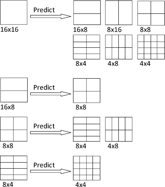
1.IntroductionH.264 is an advanced video coding standard. Its high performance in coding is associated with its high computational complexity. The standard supports seven modes of different block sizes for motion estimation (ME), which include the 16 × 16 block size and its subpartitions. We did extensive work to analyze the statistics of the mode decision results. If quantization parameter (QP) is set to 28, >60% of the macroblocks (MBs) in many sequences are encoded as 16 × 16 blocks after all modes are checked. A large amount of the computation did not provide a better result. This is illustrated in Sec. 2.1. These results shine some light on how we can accelerate variable block-size motion estimation. Although there are many fast ME algorithms in the literature, which are designed for the traditional ME structure with only one block size (16 × 16),1, 2, 3, 4, 5, 6, 7, 8, 9 and there are some fast variable block-size ME algorithms.10, 11, 12, 13, 14, 15 Some fast variable block-size ME algorithms may check 16 × 16 with 8 × 8 first, then make early mode decision with the cost of 16 × 16 and 8 × 8 modes,16 whereas in this paper, we propose to form an efficient variable block-size motion estimation algorithm that can make use of motion information and the relationship of the search results of different modes. Subpixel refinement can greatly improve the performance of motion estimation both in terms of compression ratio and quality of the decoded image. However, the ratio between the time spent on fast integer-pixel search1, 2, 3, 4, 5, 6, 7, 8, 9 and full position subpixel refinement (with partial distortion search strategy) could be nearly 1:6. The cost of this much computational time makes the subpixel refinement too costly. Some fast subpixel ME algorithms are available in the literature. One possible method is to perform an interpolation-free subpixel ME,17, 18 while another possible way is to do a candidate reduction subpixel ME,19, 20 and there are also some algorithms that use the subpixel motion vector (MV) of large block sizes to predict the subpixel motion vector of small block sizes.21 The interpolation-free subpixel ME algorithms use the ME cost of neighboring integer-pixel positions and a parabolic model to form the distortion surface of subpixel resolution positions, from which the best-match subpixel position can be found without image interpolation. In the candidate reduction subpixel ME algorithms, the ME cost of neighboring integer-pixel points is used to pick some subpixel positions as candidates, then, only these candidate subpixel positions will be checked. The accuracy of the interpolation-free subpixel ME is very close to a full position subpixel ME algorithm, but it still requires quite heavy computational time. On the other hand, the increase in bits of the candidate reduction subpixel ME algorithm is obvious, although its speed is faster. The computational complexity of Ref. 21 is between that of Refs. 19 and 20. However, although Ref. 21 can save some subpixel search computation for the partition modes, full position subpixel ME must generally be done for the 16 × 16 block. The overall computational burden appears to be >16 times more in terms of the SAD calculation. After careful observation, we find that the additional prior knowledge about the video sequence being coded can improve the search speed with little degradation on the search result. Also, the intermediate search results are extremely useful to speed up the estimation process of our algorithm. In this paper, we design a new scheme making much better use of motion information as the prior knowledge so that the algorithm can achieve a more efficient performance and be adaptable to different sequences. The motion information includes distortion values, statistical distortion distribution, motion vectors, block classification of MBs, distribution of macroblocks for different classes in the previous frame, and intermediate integer-pixel and subpixel ME results in the current frame. The rest of this paper is organized as follows: In Sec. 2, we show our analysis of the relationships of the ME results of different block sizes, mode decisions, subpixel MEs, and of checking points. Then, in Sec. 3, a comprehensive scheme trying to optimize the subpixel precision variable block-size ME is given. In Sec. 4, we illustrate the results of our experimental work, and in Sec. 5 we conclude the important points of this paper and make elaborate on our further work. 2.Analysis2.1.Relationship of Motion-Estimation Results of Different Block Sizes2.1.1.Statistics of inter- and intramodes and computation analysisThe ME of H.264 supports four intermodes that correspond to block sizes of P16 × 16, P16 × 8, P8 × 16 and P8 × 8. Each of the P8 × 8 blocks can be further subpartitioned into 8 × 4, 4 × 8, and 4 × 4 blocks. Besides the intermode, the H.264 also supports intramode coding for macroblocks in an intercoding slice, which means the encoder checks the intramodes after the best intermode is selected and then chooses the best mode from all these modes. Let us examine the distribution pattern of the intramode and fout intermodes of some typical sequences. The QP used in this analysis is 28. These include 18 sequences: “clarie,” “akiyo,” “mother and daughter,” “hall,” “silent,” “highway,” “container,” “erik,” “paris,” “foreman,” “football,” “waterfall,” “coastguard,” “bus,” “tempete,” “stefan,” “flower,” and “mobile.” Figure 1 shows our experimental results, which are the averages of the distribution data of intra- and intermodes of all test sequences. As shown in the Fig. 1, the chance to choose a block type of P16 × 16, P16 × 8, P8 × 16, P8 × 8, and Intra are 69.40, 7.28, 6.90, 14.03, and 2.39%, respectively. 2.1.2.Motion vector prediction from other block mode sizesGeneral speaking, the motion vector can reflect the motion direction of a moving object in a video sequence; thus, the motion vectors of large block sizes should be helpful for motion searching on the small block sizes, especially for some close and related modes, such as 16 × 8 mode is a close mode to 16 × 16 mode. This fact is now being used in the ME module of H.264 reference software. The method is that the motion vector of the 16 × 16 mode is used as a predicted motion vector for all other modes; the motion vector of the 16 × 8 mode is used as a predicted motion vector for the 8 × 8 mode; the motion vector of the 8 × 8 mode is used as a predicted motion vector for 8 × 4 and 4 × 8 modes; and the motion vector of the 8 × 4 mode is used as a predicted motion vector for the 4 × 4 mode, as shown in Fig. 2. This prediction strategy makes use of the relationship among motion vectors of different modes so that it could make the variable block-size ME algorithm more efficient. In order to accelerate the variable block-size ME further, we explored the relationship between mode decision results of the two stages of ME, and from this we have designed our mode prediction strategy. 2.1.3.Relationship between temporal best mode and final best mode in the mode decisionIt is obvious that motion vectors of different block sizes are related to each other. The question is how to make use of this simple observation. In our algorithm, we use 16 × 16 block size for the search in the first stage, then 16 × 8 and 8 × 16 block sizes, and 8 × 8 block size and the other partitions in the third stage. If P16 × 16 is the best mode among P16 × 16, P16 × 8 and P8 × 16, it means that a big block size is selected from among the three modes. This indicates that the moving object is probably not smaller than P16 × 16, and the chance to choose a mode even smaller than P16 × 8 and P8 × 16 is low. If this assumption is true, then modes in the third stage can be skipped and the P16 × 16 mode can be selected as the best mode. We may then save a substantial amount of computation on 8 × 8 mode and its subpartitions. The results of our experimental work are shown in Table 1, which is divided into two columns. The first column shows the cases where a small block size has been selected in the first two stages (P16 × 8 or P8 × 16), and subsequently, a smaller block size (P8 × 8) is found to be better in the third stage. The first subcolumn gives the number of macroblocks, and the second subcolumn gives the percentage of macroblocks resulting from the respective conditions. The second column shows cases to the contrary, where a large block size has been selected in the first two stages (P16 × 16), but after the third stage, a small block size (P8 × 8) is chosen as the best one among all intermodes. Each of these two columns is divided into two subcolumns; one is the number of macroblocks in the corresponding cases, whereas the other is the percentage. (The QP used in this analysis was 28.) From the data in Table 1, we can see that, for most sequences, the intermediate mode decision results are usually consistent with the final mode decision results. Hence, we can make use of this fact to formulate our mode prediction strategy. Table 1Chance to choose P8 × 8 mode when a P16 × 16, P16 × 8, or P8 × 16 mode is selected.
2.2.Relationship between Mode Decision and Subpixel Motion Estimation2.2.1.Why do we need subpixel motion estimation?There are many reasons why subpixel ME can enhance the performance of ME by eliminating the temporal redundancy, as follows:
According to our experimental results of 18 standard test sequences with QP = 28, the compression ratio and the peak signal-to-noise ratio (PSNR) of the decoded videos are 28 and 36.76 dB for the encoding process, using a ME algorithm with only integer-pixel search, whereas they are 50 and 37.01 dB for the encoding process with both integer-pixel search and subpixel refinement. Hence, subpixel refinement can greatly improve the performance of ME in terms of both compression ratio and decoded image quality. 2.2.2.Why do we need variable block-size motion estimation?A moving object may spread among several MBs. On the other hand, in one MB there may be more than one object. If we perform ME with only a 16 × 16 block size, then we may not find the best match for any of the objects in the block. To solve this problem involves H.264 variable block-size ME, which is a key feature of our investigation. 2.2.3.Mode decision not dependent on subpixel motion estimationIdeally, mode decision is made after completion of integer-pixel ME and subpixel ME of all modes. This is time consuming. In order to save time, we may make mode decision after the completion of integer precision ME of all modes. Table 2 gives our experimental results on this issue, which shows that subpixel ME does not change the result of the mode decision in most cases. Hence, even though the subpixel ME is an essential part for a precision ME, it can be done after the mode decision is made. Table 2Comparison of the results of making mode decision after (i) subpixel precision and (ii) integer pixel precision ME.
We have also inspected the relationship of the mode decision and subpixel ME from another point of view. This is to examine the bits spent on motion vectors, modes, and residual errors in the bit stream coded with (i) mode decision made after subpixel ME and (ii) mode decision made after integer-pixel ME. In both cases, both integer and subpixel ME were carried out. However, in case (ii) mode decision was made after making the integer-pixel ME of all possible modes, which saves much computation compared to case (i), because in this case, subpixel ME is only required to be carried out for the selected mode. Table 3 shows our experimental results, in which “MV bits” means bits spent on motion vector, “Mode bits” means bits spent on block mode, “Coeff bits” means bits spent on residual error, “Others bits” means bits spent on slice head, δ-quantization parameter, and “Intrabits” means bits spent on intrablocks in the intercoded frames. Table 3Bits consumption for two mode decision strategies.
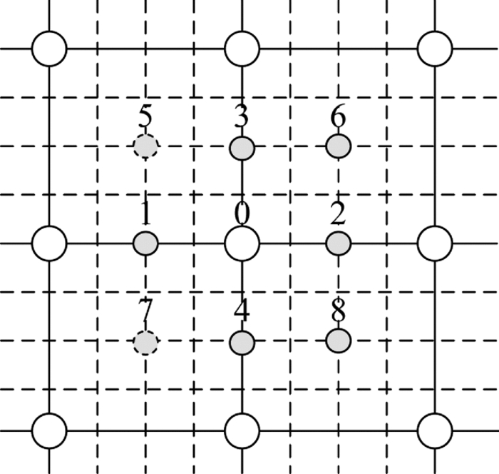
It is interesting to note from Table 3 that although the mode decision was made after subpixel ME, case (i) requires lower MV bits (339,017 bits) and Mode bits (179,341 bits); yet case (ii) for which the Mode decision was made after integer-pixel ME only requires fewer Coeff bits (2,595,426 bits) than that in case (i) (2,902,317 bits). Consequently as an overall result, case (ii) requires fewer bits than case (i) on average. Hence, different from the conventional approach (such as that used in H.264 JM12.2), we prefer to make a mode decision after integer-pixel ME, which requires one to perform subpixel ME for only the best mode; hence, it reduces computational effort substantially. 2.3.Relationship among Candidate Checking Points of Half-Pixel Motion EstimationCorrelation is widely used to reveal the relationship among signals from different sources. Let us also make use of this mathematical tool and calculate the correlation coefficients of half-pixel point pairs to reveal the relationship among them. Recall that the correlation coefficient, ρX,Y, between two random variables X and Y is defined as follows: Eq. 1[TeX:] \documentclass[12pt]{minimal}\begin{document}\begin{equation} \rho _{X,Y} = \frac{{{\mathop{\rm cov}} (X,Y)}}{{\sigma _X \sigma _Y }} = \frac{{E[ {(X - \mu _x)(Y - \mu _y)} ]}}{{\sigma _X \sigma _Y }},\end{equation}\end{document}In Fig. 3, integer-pixel locations are indicated by big circles, whereas half-pixel locations are indicated by small circles. Let us label eight nearby half-pixels of the best integer pixel 0 as half-pixel points 1,2,…,7. Each half-pixel point of 0 can form seven pairs of half-pixels: Pair 1 to pair 7, with the rest of the half-pixel points, as indicated in Fig. 4. In our experimental work, after the best integer location was found for each block, the correlation coefficients of its corresponding pairs—Pair 1 to pair 7—were calculated with Eq. 1. The values of these seven half-pixel correlation coefficients were added, respectively, to seven accumulators for all block locations and mode–type positions (including 16 × 16, 16 × 8, 8 × 16, 8 × 8, 8 × 4, 4 × 8, 4 × 4). We accumulated the seven correlation coefficients of all blocks in 150 frames of each test sequence, respectively. The seven values shown in Fig. 5 are the average values of 18 sequences, in which the vertical axis indicates the accumulated values of the correlation coefficients and the horizontal axis indicates pair numbers. This statistical result shows that the accumulated values of correlation coefficients are consistent with the distance between the two points of a pair. That is, if the distance is shorter, it is more correlated. Hence, in our algorithm, the eight half-pixel points are grouped into near-neighbor points and far-neighbor points according to the distance between the half-pixel point and the best integer point. Let us define that points 1–4 are near neighbors because they are closer to the best integer-pixel position compared to points 5–8, which are far neighbors. Each far neighbor point is on the perpendicular bisector of two near-neighbor points. The search results of the far-neighbor points are supposed to be related to that of the near-neighbor points. Further experimental work was done to check whether the risk of missing the best match point is worth taking, and its results are shown in Table 4. Table 4Risk of missing the best match point.
We trust that the idea of directional tendency will work for subpixel ME, which is only to make necessary tests on locations along the direction indicated by the search path, and this idea should work even better than that for integer-pixel ME.7 We have verified this idea with the following experimental work in order to avoid the risk missing important locations. We checked the four near neighbors, collected the results, and then checked the four far neighbors and counted the number of half-pixel ME operations required in a counter, counter1. If the best near-neighbor point was 3 for example, and the best far-neighbor point was 7 or 8, we increased the number of contradictions in another counter, counter2. This gives the number of times we got a half-pixel motion vector, which has an opposite direction to the search result of near neighbors. The total number of half-pixel ME and the number of contradictions are shown in columns (2) and (3), respectively, of Table 4. The ratio between columns (3) and (2) is shown in column (4), which indicates that the directional information obtained from the search result of near-neighbor points is reliable. 2.4.Relationship between Half- and Quarter-Pixel Motion-Estimation ResultsHalf-pixel ME and quarter-pixel ME are usually used to refine the integer-pixel ME result. Half-pixel refinement is conducted on neighbor points surrounding the best integer-pixel point. The best half-pixel point will then be the center for quarter-pixel refinement, which may not be the original center point of half-pixel refinement. Hence, the quarter-pixel motion vector should not be predicted from only a half-pixel motion vector. It is found7, 8 that block classification is an effective way to determine whether or not a macroblock belongs to the same moving object as its neighboring MBs. It provides a noticeable improvement in the integer-pixel ME algorithm. Is it possible to combine the block-classification result of the previous frame and the half-pixel ME result to make an early termination before the quarter-pixel ME? According to the block classification, we can predetermine the current MB as an ordinary block or a special block. If we predetermine it as an ordinary block, then it indicates that the current MB probably belongs to the same moving object as its neighboring MBs. The blocks that belong to the same moving object should have similar or even the same motion vector. The motion of a moving object within a small set of consecutive frames should be consistent. Hence, we suppose if the current block is part of a predetermined ordinary macroblock, then its colocated macroblock has a zero motion vector, and the motion vector of the current block after half-pixel refinement is also zero. The current block is then most likely to be a stationary block, and it will also get a zero motion vector after quarter-pixel refinement. In our experimental work, we calculated the chances of getting a zero vector or nonzero vector after a quarter-pixel refinement when the condition to predict the current block as a stationary block is true. The results of our experimental work listed in Table 5 verify that our assumption is true, which means that the chance of missing a valid quarter-pixel motion vector is usually not high. Table 5Chance to ignore an existing quarter-pixel MV.
3.Algorithm Development3.1.Motion Information for Early Termination and Early Mode Decision3.1.1.Block classification according to variable block size motion informationOur block classification is designed to imply the motion characteristic of macroblocks so that we can apply fast strategies to macroblocks (and their subpartition blocks) with certain features. As a recent practice, during the ME procedure for only 16 × 16 blocks, the motion vectors of neighboring MBs were used to predict the motion vector of the current MB before the pattern search stage. Then, the pattern search starts from the point indicated by the best-predicted motion vector. After the pattern search stage, if the final motion vector is not the same as the best-predicted motion vector, then the macroblock may contain a different moving object from its neighboring MBs; thus, we classify it to fall into the special macroblock group (group S), whereas the other macroblocks (with the same MV) are classified into the ordinary macroblock group (group O). In this scheme, for ME with variable block sizes, we have seven groups of “the best” predicted motion vectors corresponding to seven block sizes. Among the best-predicted motion vectors of the seven partitions, only those of the best mode are used in the block-classification process. If the best mode is classified as belonging to the special block group, then the current macroblock is set as a special MB. Whether it is a “special MB” and an “ordinary MB” of a MB in the current frame can be “predetermined” according to the block classification of the previous frame. For a special MB in the previous frame, its colocated MB and its eight surrounding MBs are predetermined as special MBs, and others are predetermined as ordinary MBs in the current frame. Hence, the classification method works well in the variable block-size ME scheme. 3.1.2.Distribution of best mode SAD values of macroblocks in successive framesMotion continuity exists not only on neighboring areas in one frame but also among successive frames. If the sum-of-absolute-differences (SAD) statistics of successive frames are similar to each other, then the statistical distribution of SADs of the current frame can be predicted by the SAD statistics of the previous frame. This appears true for ME with 16 × 16 blocks. For variable block-size ME, can we find a similar correlation? The SAD of a macroblock in variable block-size ME is composed of the SAD of each block in the current macroblock and its corresponding best match block in the reference frame. In Fig. 6, SAD represents the SAD values of the best mode of each of the macroblocks in frames 3–5 of the foreman sequence. Because most of the SAD values of these frames are distributed within the range 0–2000, only SAD values in this range are shown in Fig. 6 for illustration. These values are divided into 16 groups (bins). The numbers of macroblocks having SAD values larger than the minimum values of groups are plotted on the graph by dots. In Fig. 6, it is clear that the SAD statistics of the three frames are similar to each other. We have found similar patterns on other consecutive frames making use of this analysis with other test sequences (such as hall and football video sequences), with slow and fast motion activities. Hence, we can make a prediction on the statistical SAD distribution of the current frame from that of the previous frame. The method is to let the SAD statistics of the previous frame be the predicted SAD statistics of the current frame before ME and update it with the real SAD statistics of the current frame after ME. The predicted SAD statistics of the current frame can help us to find an effective threshold to be used in the next frame. After checking all the predicted motion vectors, we may compare the SAD value of the best-predicted motion vector to the threshold to make a decision on the early termination of one mode. This strategy makes it possible for us to skip further searching for some predetermined ordinary macroblocks after the motion vector prediction. This is the same approach as the one for which we can do for ME with 16 × 16 blocks. It can also have a good effect on the variable block-size ME because this allows us to choose early termination before the pattern search of each mode. In this way, we can reduce the computation time spent on pattern search. If the pattern search is skipped, then the final MV of the block will be the same as its best-predicted MV. Subsequently, the block will become an ordinary block after ME of the current frame. It means early termination generates more ordinary MBs. It is necessary to control the number of blocks chosen for early termination in order to maintain the performance of the ME algorithm. Hence, we need to control the threshold for early termination. From experimental work, we note that the number of ordinary MBs of the successive frames do not change much. Thus, we expect that the number of ordinary MBs in the current frame be similar to that of the previous frame. Experimental evidence shows us that the number of ordinary macroblocks in the current frame is closely related to the threshold for early termination. The threshold can be obtained according to the predicted number of ordinary MBs of the current frame. Hence, in our design we find the threshold for early termination by looking up the SAD value-number distribution graph of macroblocks (as shown in Fig. 6) of the previous frame, which is a prediction of the current frame. The SAD value corresponding to the number of ordinary macroblocks in the previous frame is taken as the threshold required. In this example, we divided the range into 16 groups. If the threshold is too low, then this fast strategy may not work. Furthermore, an unexpectedly higher threshold could compromise too much the precision of the search. Hence, we suggest an upper bound and lower bound for the threshold, which are 800 and 1500, respectively, according to the results of a large number of experiments. The block classification and threshold calculation have been designed in such a way that they are suitable for variable block-size ME. 3.2.Eliminating Subpixel Motion Estimation of All Unselected ModesBecause mode decisions do not depend on the subpixel ME, we can consider them as two separate problems and deal with them individually. This means that we can perform integer-pixel ME for each mode, choose the best mode according to their rate distortion values, and then perform subpixel ME for only the best mode from the point given by the motion vector of the best integer mode, as shown in Fig. 7. 3.3.Fast Subpixel Strategies of One Mode3.3.1.Directional search strategy for subpixel motion estimationLet us use the analysis results in Sec. 2.3 to accelerate the full-position subpixel ME algorithm. The full-position subpixel ME with early termination strategy has been used in the JM model of H.264. It contains two consecutive steps: half-pixel refinement and quarter-pixel refinement. Half-pixel refinement needs to examine all eight half-pixel checking points surrounding the best integer point, and the quarter-pixel refinement needs to examine eight quarter-pixel checking points surrounding the best half-pixel point. It must calculate the SAD of subpixel positions 16 times. According to our experimental work the additional time required by this algorithm is nearly six times that of the time spent on our fast integer-pixel search procedure. The relationship among candidate positions of the half-pixel ME shows that we can rely on the directional information obtained from the search result of near-neighbor points to skip some of the far-neighbor points before we examine them (see Sec. 2.3). Let us refer to Fig. 3 for our fast half-pixel ME process. There are eight half-pixel points surrounding the integer pixel 0 (i.e., points 1–8). Step 1: We need to examine the four near-neighbor points surrounding the best integer-pixel point, 1–4. Let us keep the motion vector and minimum SAD value of the best point as the temporal half-pixel ME result. Step 2: If one of the four near-neighbor points is better than the best integer-pixel point, we examine the two far-neighbor points besides the best near-neighbor point. For example, if the best near-neighbor point is point 2, then points 6 and 8 will be examined. If a smaller SAD is found, then it will be stored as the minimum SAD and the motion of this point (i.e., the displacement between the best integer-pixel point and this point) will be set as the half-pixel ME result. Otherwise, we set the temporal result in step 1 as the half-pixel ME result. Note that the two points encircled with a dashed line will not be examined in this fast refinement. This candidate rejection strategy is also applied to quarter-pixel refinement in our algorithm. 3.3.2.Stationary block identification with the result of half-pixel motion estimation; and skipping quarter-pixel motion estimation for stationary blocksIn this part, the relationship between half- and quarter-pixel ME results will be combined with the prior knowledge of MBs in the previous frame to form a stationary block-identification strategy to skip the quarter-pixel ME for the stationary blocks. This is to accelerate further the subpixel ME algorithm. If we find that the current block is a part of a predetermined ordinary MB and the motion vector of its co-located MB in the previous frame is a zero vector, then we may assume that the current block belongs to the same stationary object as its neighboring MBs. If the motion vector of the current block is a zero vector after half-pixel refinement (i.e., the condition for stationary block identification is true.), then it is more likely that the current block will have a zero motion vector after quarter-pixel refinement. Hence, we can consider skipping the quarter-pixel refinement of the current block. 3.4.Overall Structure of the AlgorithmFigure 8 shows a flowchart of the proposed approach. There are five major modules of operations in the structure, which are integer-pixel ME, intraprediction, mode decision, subpixel ME, and motion-information collection. The integer-pixel ME includes motion search for variable block sizes. The first stage of module one is to search for the 16 × 16 block size; then in the second stage, the macroblock is divided into 16 × 8 or 8 × 16 blocks to carry out a motion search on the small blocks, individually. In the third stage, the macroblock is further divided into 8 × 8, 8 × 4, 4 × 8, and 4 × 4 blocks. After checking the intermodes, the intraprediction is then considered. There is one conditional execution for “early termination” in each stage (not shown on Fig. 8 for stages 2 and 3). And there are “early mode decision1” and “early mode decision2” after stage1 and stage2, respectively. The early termination check is carried out after checking all predictors that are motion vectors of the neighboring MBs in the spatial and temporal domains. 3.4.1.Condition for early terminationThe conditions for early termination are as follows:
Note that if the current block is a subpartition of a MB, then we will then scale the threshold value appropriate to the size of the current block. For example, if the current block is an 8 × 8 block, the original threshold is 800. We then have to compare the current SAD with (800*8*8)/(16*16) = 200 to make the decision for early termination. The scale factor will also be used for this block to form an appropriate threshold to assist fast mode decisions. If the conditions are true, early termination will become effective, which means the best predicted motion vector (PMV) is selected as the final MV of the current block. The pattern search part is then skipped for this mode, and the ME process will move onto another mode with similar or smaller block sizes. 3.4.2.Condition for early mode decisionThe conditions for “early mode decision1” are as follows:
Hence, if early mode decision1 is selected, P16 × 16 is set to the best mode of the current MB and all the other modes are skipped. Otherwise, we will check 16 × 8 and 8 × 16 modes in stage 2. At the end of stage 2, if we find that P16 × 16 is the best mode among P16 × 16, P16 × 8 and P8 × 16, this forms the condition for early mode decision2. If this condition is true, then P16 × 16 is selected as the best mode and P8 × 8 and its subpartition block sizes are not considered. After all inter- and intramodes are checked, the best mode will be selected in the mode decision module. If the intermode is selected, the subpixel ME is then carried out on the selected best mode. There is also a chance for early termination (not shown in Fig. 8) after the half-pixel ME process in the subpixel motion-estimation module. The conditions for this early termination are as follows:
The subpixel ME may be done on a subpartition mode of a P16 × 16 macroblock because the best mode can be any one of the four modes. Moreover, the fast directional approach can be used no matter whether the subpixel ME is conducted on an MB or a block. The search process is then completed for a macroblock at this stage. In the next module, the motion information of the MB is calculated and stored to form the statistical motion information of the current frame, which will be used as prior knowledge to guide the ME procedure of the next frame. If the PMV of the current MB is equal to its final MV in the best mode, then the current macroblock is classified into the ordinary MB group and the number of ordinary MBs increases by 1. Then, the minimum SAD value of the MB is recorded. If an MB with its best possible mode consists of several blocks, then the SAD values of these blocks are used to form the SAD of this MB, possibly with the minimum value. If all MBs have been processed, then the statistical motion information of the frame is obtained, and thresholds for early termination and the early mode decision for the next frame will be generated from the result of the statistics. The SAD values of all MBs are examined. The range of these SAD values is divided into 16 parts according to their values. Subsequently, as shown in Sec. 3.1.2, a new SAD value–number distribution is formed, which can be used to find the threshold for early termination by looking for the SAD value corresponding to the number of ordinary MBs of this frame. This is stored inside “the motion-information collection module” to be used in the next frame. Note that both integer-pixel motion search and subpixel motion search processes of the algorithm make use of directional motion search. Further details of the directional integer-pixel ME is illustrated in Ref. 7, whereas the directional subpixel ME method is given in Sec. 3.3.1 of this paper. 4.Experimental ResultsThis fast subpixel precision variable block-size ME algorithm consists of three groups of fast strategies: a fast variable block-size ME strategy, an effective way to eliminate subpixel ME of all unselected modes; and a fast subpixel ME strategy. In this section, we will illustrate the results of our experimental work. We will initially make an analysis and verify the improvement of these three groups of our fast strategies independently. We then compare the performance of our fast variable block-size and subpixel ME strategies to exiting algorithms, and show the overall performance of our work compared to other algorithms in the literature. The software was the JM12.2 encoder. The proposed algorithm is combined with the mode selection procedure of the H.264 reference software (JM12.2) to improve the speed of ME so as to enhance the efficiency of the encoder. We used an IBM Notebook with Inter Core 2 Duo CPU T7300 2.0G and 2-gigabytes of RAM. The ME search range was 32. The QP was set to 28. The RDOptimization option was set to 1, which is the high complexity mode. There were 18 test sequences with the common image format (CIF) used in our experimental work. Only the average values of the computation time (in seconds) of the experimental results are given as shown in Fig. 9. The abbreviations of this graph are as follows: “Int” stands for our fast integer-pixel ME;7 VBS is variable block-size ME; “sub” is subpixel ME; “No” means the function is not used [e.g., “No_VBS_sub” means subpixel precision ME without variable block-size function, and this implies that it supports 16 × 16 block size only (without using VBS)], and F represents that our fast strategies of the function were used (e.g., “FVBS_sub” means fast variable block-size ME with subpixel refinement on each mode). The y-axis of the graph shows the ME time in second. The number on the top of each block gives the average ME time for each scheme. We use four matrices in the form of ratios to make an analysis and to reflect the accuracy of our measurements, Eq. 2[TeX:] \documentclass[12pt]{minimal}\begin{document}\begin{equation} r_1 = \frac{{{\rm METime(FVBS\_sub)}}}{{{\rm METime(VBS\_sub)}}} = \frac{{9.42\,\,{\rm s}}}{{25.38\,\,{\rm s}}} = 0.3712, \end{equation}\end{document}Eq. 3[TeX:] \documentclass[12pt]{minimal}\begin{document}\begin{equation} r_2 = \frac{{{\rm METime(FVBS)}}}{{{\rm METime(VBS)}}} = \frac{{X_1 \,\,{\rm s}}}{{3.91\,\,\,{\rm s}}} \approx 0.3712. \end{equation}\end{document}Let us define the third and fourth ratios, Eq. 4[TeX:] \documentclass[12pt]{minimal}\begin{document}\begin{equation} \begin{array}{l} \displaystyle r_3 = \frac{{{\rm METime(VBS\_Fsub\_only)}}}{{{\rm METime(VBS\_sub\_only)}}} \\[12pt] \,\,\,\,\,\displaystyle = \frac{{{\rm METime(VBS\_Fsub)} - {\rm METime(VBS)}}}{{{\rm METime(VBS\_sub)} - {\rm METime(VBS)}}} \\[12pt] \,\,\,\,\, \displaystyle = \frac{{16.55 - 3.91\,\,{\rm s}}}{{25.38 - 3.91\,\,{\rm s}}}\, = \frac{{12.64\,\,{\rm s}}}{{21.47\,\,{\rm s}}} = 0.5887, \\ \end{array} \end{equation}\end{document}Eq. 5[TeX:] \documentclass[12pt]{minimal}\begin{document}\begin{equation} \begin{array}{l} \displaystyle r_4 = \frac{{{\rm METime(No\_VBS\_Fsub\_only)}}}{{{\rm METime(No\_VBS\_sub\_only)}}} \\[12pt] \,\,\,\,\, \displaystyle = \frac{{{\rm METime(No\_VBS\_Fsub)} - {\rm METime(Int)}}}{{{\rm METime(No\_VBS\_sub)} - {\rm MET}{\rm ime(Int)}}} \\[12pt] \,\,\,\,\, \displaystyle = \frac{{X_2 - 0.20\,\,{\rm s}}}{{3.08 - 0.20\,\,{\rm s}}} = \frac{{X_3 \,\,{\rm s}}}{{2.88\,\,{\rm s}}} \approx 0.5887, \\ \end{array} \end{equation}\end{document}Table 6 shows the performance comparison of full search (FS), enhanced predictive zonal search (EPZS), fast variable block-size ME algorithm in Ref. 14 (FORMER) and our fast variable block-size ME strategy (PRES). Both FS and EPZS are given by JM12.2.22 All four algorithms were done without subpixel refinement at this stage. Table 6 shows the FORMER algorithm is slightly faster than EPZS, while our variable block-size strategy can achieve much faster speed than FORMER with similar PSNR and bits per pixel performance as the FS and EPZS. Table 6Performance comparison of variable block-size ME algorithms.
Table 7 shows the performance comparison of full-position subpixel ME search, our proposed fast subpixel ME strategy, interpolation free subpixel ME,16, 17 and fast fractional PEL (picture element) ME.18 All of them were done with fixed block size: 16 × 16. The computational complexity of interpolation free subpixel ME algorithm is similar to that of the full-position subpixel ME search, so it has less degradation on PSNR. The fast fractional PEL subpixel ME has a faster speed and a PSNR degradation of 0.05 dB. However, it has a significant bit-rate increase of 11.63%. Among them, the present of our fast subpixel ME strategy has almost the same PSNR (36.93 dB) and a very slight increase in bit-rate (0.53%) performance as compared to the full position subpixel ME algorithm, and it has a relatively high speedup factor (i.e., 1.62 times of the full position subpixel ME speed). Table 7 shows the experimental results of the 18 sequences arranged according to the motion activities of the sequences from low to medium to high values. Again, let us explain the abbreviations used in the table, which reflect the performances of different versions of our algorithm, as follows: Table 7Performance comparison of subpixel ME algorithms (with fixed block size: 16 × 16).
“No fast VBS, no SubPEL, no fast SubPELME” means subpixel precision variable block-size ME without fast strategies. “Fast VBS, no SubPEL elimination, no fast SubPEL ME” means subpixel precision variable block-size ME with fast strategies for making mode selections (see Sec. 3.1). “No fast VBS, SubPEL elimination, no fast SubPEL ME” means subpixel precision variable block-size ME with the subpixel ME elimination method (see Sec. 3.2). “No fast VBS, no SubPEL elimination, Fast SubPEL ME” means subpixel variable block-size ME with fast strategies on subpixel ME (see Sec. 3.3). “PRES” means the present algorithm, which is the final version of our algorithm, and these results were found by making use of all three groups of our fast strategies. The final version of our algorithm (PRES) is composed of fast variable block-size ME strategy, subpixel ME elimination strategy, and fast subpixel ME strategy. It is compared to the full-search ME algorithm and the EPZS. Both FS and EPZS are given by JM12.2.19 The FS algorithm includes the VBS full search integer-pixel ME and the full-position subpixel refinement. The EPZS is composed of the fast VBS integer-pixel ME and subpixel refinement with a fast termination strategy using JM12.2. All algorithms used a SAD function for evaluation with a partial distortion search method as the basic technique. The performance comparison includes PSNR, Bits per pixel, and Speedup (real time), where PSNR means the average PSNR values of the luminance component of the decoded frames. “Bits per pixel” gives the number of bits to code 1 pixel on average while the number of frames was set to 150 for all sequences. “Speedup (real time)” is the ratio between ME time of the FS and the ME time of the respective fast algorithms being considered. (The computational time of one algorithm for one test sequence was obtained from the average of 12 executions. After the executions, two higher values and two lower values were deleted. Then the average value of the eight values that remain is the required computational time.) Furthermore, Table 8 gives the performance of five versions of our algorithm. The PSNR and bits per pixel do not change much while the speedup increases from 13, 20, 35, 49, to 60 as compared to the full-search algorithm with subpixel refinement and termination strategy. This matches Fig. 9, which also shows the speedup improvement made by using our fast variable block-size strategies and fast subpixel ME strategies, respectively. Table 8 clearly shows the effect of subpixel ME elimination among various modes. A speedup of 49 is achieved by this strategy, which confirms its significance in our subpixel precision variable block-size ME scheme. Table 8Performance comparison of ME algorithms.
If we compare the PSNR values of the full search and EPZS of each sequence, it is not difficult to find that the PSNR values of EPZS are lower than those of the full search for 13 sequences. It has the same PSNR value with the Full Search for three sequences and higher PSNR values for two other sequences. The PSNR values of UMHexagonS are lower than that of the full search for 11 sequences, the same as that of the full search for six sequences, and higher for ine sequence. However, when we compare the PSNR of the full search to the proposed algorithm, we can see that the proposed algorithm has lower PSNR values for nine sequences and the decreases vary from 0.01 to 0.11, while it has higher PSNR values for the other nine sequences and the increases also vary from 0.01 to 0.11. Hence, it is not surprising that the average PSNR of the proposed algorithm is the same as that of the full search. For bit-rate performance, all the three fast search algorithms (EPZS, UMHexagonS, our algorithm) have a similar bit-rate performance as that of the full search. Besides PSNR and bit rate, the proposed algorithm is much faster than the full search, UMHexagonS and EPZS. There is speedup of 60 times faster than the speed of full search, five times faster than the speed of EPZS, and four times faster than the speed of UMHexagonS. The speedup value varies from 38 to 78 as compared to the full search. If the motion in a sequence is mainly translational, then the speedup ratio is usually high, even without degradation or a decrease in PSNR. This is the situation for the bus sequence, for example, as shown in Table 8. The proposed algorithm is also efficient for using other QP values. Table 9 gives the performance comparison among FS, UMHexagonS, EPZS, and the proposed ME algorithm using different QP values. Each entry in Table 9 was obtained from 12 sequences (three sequences with the format 176 × 144 and nine sequences with the format 352 × 288). From Table 9, we can see that the proposed algorithm can always achieve very similar PSNR and bits-per-pixel performance compared to the FS. It has a noticeably higher speedup value than that of the EPZS (or UMHexagonS) as shown in Table 8. For a high-QP condition, the speedup value decreases slightly (for example, the speedup value changes from 54 to 46 for varying the QP from 30 to 38, respectively). The reason for this is that the image distortion may become serious with a high-QP condition. The acceleration strategies based on our analysis of the motion characteristics of successive frames are affected by the image distortion. This is a compromise that we have to pay for a guarantee of the video quality of the encoded sequence. Table 9Performance comparison of ME algorithms.
We have also made an evaluation of our algorithm using some high-definition video sequences as shown in Table 10. Five sequences with a resolution of 1920 × 1080 were tested. These include CrowdRun and ParkJoy sequences, which are two motion-intensive sequences; DucksTakeOff sequence, which has irregular water wave motion; and InToTree and OldTownCross sequences, which contain both zoom and translation motion activities. All these sequences contain plenty of image details. Results of this experimental work show that our algorithm has nearly the same PSNR as the FS, and the bit-rate performance is also very similar. However, the speedup ratio of our algorithm compared to the FS is 56, which is substantially higher than the speedup value of EPZS. This speed performance is similar to that achieved in lower resolution video sequences. Table 10Performance comparison of different algorithms, VM: JM12.2.
In some of our experimental results, the performance of the present approach appears, in terms of both PSNR quality and bit rate, better than the full search. It is due to the inaccuracy of the RD evaluation of the JM software, which cannot optimize all factors simultaneously. In principle, the evaluation should give us the best trade-off among motion-vector size, residual signal, intra- and intermode selection, mode-type selection, etc. Actually, the optimization can be done, generally, but not too ideally, and this is a very good topic deserving for much further researh in the future. Figure 10 shows the accumulated bits distribution of 18 standard test sequences using the present approach (PRES) or FS ME algorithms with QP equal to 28. The FS working under the rate distortion (RD) evaluation can automatically acquire shorter motion vectors, but more “Intra bits” are required, for example. This also results in that more “Coeff bits” of the FS being required as compared to that of PRES. Hence, the “Total bits” of PRES is lower than FS. This is just an example to explain the reason that PRES can achieve lower bits per pixel when the QP is >32, as shown in Table 9. 5.ConclusionIn many cases, there are two main reasons for making a fast ME algorithm be less efficient; namely, some promising locations may be skipped or some unnecessary searches may be continued. In the latter case, we may not even be aware that there are many unnecessary time-consuming steps in the algorithm. Each of these two types of problems will generate a certain degradation of the image quality, and the unnecessary searching will affect the efficiency. However, these are apparently two conflicting points. Usually, a smart trade-off between these two points must be achieved, or a better solution is to prevent both cases from happening. This in turn relies on a critical and yet simple analysis of the current data to make decisions for the fast algorithm. We have successfully resolved these problems by formulating our fast strategies based on the motion information of blocks in the previous frame and on their current statistics. The fast strategies are based on particular properties even at the individual block level. We have done an analysis of the statistics of the mode selection of variable block-size ME. We found that >80% of the computation does not provide a better result in the original algorithm given by JM12.2, for example. We have also done much work to analyze the relationship of the ME results of different block sizes, the relationship between mode decision and subpixel ME, the relationship among candidate checking points of half-pixel ME, and the relationship between half-pixel and quarter-pixel ME results. The analysis reveals the possibility of making early termination and early mode decisions with little damage to the search results. It also reflects the principle of fast strategies and may give clues on how fast strategies be used. The proposed new method for making early terminations and early mode selections of variable block size ME relies heavily on the motion information from all blocks and their statistical information of the successive frames. The statistical information can adaptively be updated to fit the new incoming frames. We have to make some presumptions based on the motion information and the statistics information. These conditional presumptions are very close to the real situations. Even though there are few occasional misses of the best match or misses of the best mode with our fast strategies, we have found that the degradation of image quality is not substantial at all. Results of our experimental work also show that our approach can be over four times faster than the algorithms available in the reference software of H.264 (JM12.2). Even though we have found that our algorithm is better than other algorithms available in the literature, there is still plenty of room for improvement. We may make an exploitation in a more systematic way to find out more immediate information to help us make the correct decision. We may compare the actual situation with the correctness of our decision rules. What is the percentage of decisions that are successful? How far can we trim our algorithm with >95% correct decisions yet still have an overall improvement of the new algorithm? This is a fruitful direction for further research. AcknowledgmentThis research work is supported in part by the Centre for Signal Processing (1BB87) of the Hong Kong Polytechnic University, CERG grant (B-Q07G) of the Hong Kong SAR Government and the Beijing Institute of Technology. ReferencesY.-L. Chan and W.-C. Siu,
“An efficient search strategy for block motion estimation using image features,”
IEEE Trans. Image Process., 10
(8), 1223
–1238
(August 2001). https://doi.org/10.1109/83.935038 Google Scholar
K.-C. Hui, W.-C. Siu, and Y.-L. Chan,
“New adaptive partial distortion search using clustered pixel matching error characteristic,”
IEEE Trans. Image Process., 14
(5), 597
–607
(May 2005). https://doi.org/10.1109/TIP.2005.846020 Google Scholar
A. M. Tourapis, O. C. Au, M. L. Liou, and G. Shen,
“Fast and efficient motion estimation using diamond zonal based algorithms,”
J. Circuits Syst. Signal Process., 20
(2), 233
–251
(June 2001). https://doi.org/10.1007/BF01201140 Google Scholar
Y.-L. Chan and W.-C. Siu,
“New adaptive pixel decimation for block motion vector estimation,”
IEEE Trans. Circuits Syst. Video Technol., 6
(1), 113
–118
(February 1996). https://doi.org/10.1109/76.486426 Google Scholar
P. I. Hosur and K.-K. Ma,
“Motion vector field adaptive fast motion estimation,”
(1999) Google Scholar
I. Ahmad, W. Zheng, L. Jiancong, and L. Ming,
“A fast adaptive motion estimation algorithm,”
IEEE Trans. Circuits Syst. Video Technol., 16
(3), 420
–438
(2006). https://doi.org/10.1109/TCSVT.2006.870022 Google Scholar
Y. Zhang, W.-C. Siu, and T. Shen,
“Yet a faster motion estimation algorithm with directional search strategies,”
475
–478
(2007). Google Scholar
Y. Zhang and T. Shen,
“Motion information based adaptive block classification for fast motion estimation,”
686
–691
(2008). Google Scholar
K.-C. Hui and W.-C. Siu,
“Extended analysis of motion-compensated frame difference for block-based motion prediction error,”
IEEE Trans. Image Process., 16
(5), 1232
–1245
(May 2007). https://doi.org/10.1109/TIP.2007.894263 Google Scholar
Liangming Ji and Wan-Chi Siu,
“Reduced computation using adaptive search window size for H.264 Multi-Frame Motion Estimation,”
(2006). Google Scholar
L. Yang, K. Yu, J. Li, and S. Li,
“An effective variable block-size early termination algorithm for H.264 video coding,”
IEEE Trans. Circuits Syst. Video Technol., 15
(6), 784
–788
(June 2005). Google Scholar
S. Saponara, M. Casula, F. Rovati, D. Alfonso, and L. Fanucci,
“Dynamic control of motion estimation search parameters for low complex H.264 Video Coding,”
IEEE Trans. Consumer Electron., 52
(1), 232
–239
(2006). https://doi.org/10.1109/TCE.2006.1605052 Google Scholar
Y.-W. Huang, B.-Y. Hsieh, S.-Y. Chien, S.-Y. Ma, and L.-G. Chen,
“Analysis and complexity reduction of multiple reference frames motion estimation in H.264_AVC,”
IEEE Trans. Circuits Syst. Video Technol., 16
(4), 507
–522
(2006). Google Scholar
C. Grecos and M. Y. Yang,
“Fast inter mode prediction for P slices in the H264 Video Coding Standard,”
IEEE Trans. Broadcast., 51
(2), 256
–263
(2005). https://doi.org/10.1109/TBC.2005.846192 Google Scholar
T.-Y. Kuo and C.-H. Chan,
“Fast variable block size motion estimation for H.264 using likelihood and correlation of motion field,”
IEEE Trans. Circuits Syst. Video Technol., 16
(10), 1185
–1195
(2006). https://doi.org/10.1109/TCSVT.2006.883512 Google Scholar
J. Lee and B. Jeon,
“Fast mode decision for H.264 with variable motion block sizes,”
Lect. Notes Comput. Sci., 2869 723
–730
(2003). https://doi.org/10.1007/b14229 Google Scholar
P. R. Hill, T. K. Chiew, D. R. Bull, and C. N. Canagarajah,
“Interpolation free subpixel accuracy motion estimation,”
IEEE Trans. Circuits Syst. Video Technol., 16
(12), 11519
–11526
(2006). https://doi.org/10.1109/TCSVT.2006.885722 Google Scholar
J. W. Suh and J. Jeong,
“Fast sub-pixel motion estimation techniques having lower computational complexity,”
IEEE Trans. Consumer Electron., 50
(3), 968
–973
(2004). https://doi.org/10.1109/TCE.2004.1341708 Google Scholar
Y.-J. Wang, C.-C. Cheng, and T.-S. Chang,
“A fast fractional PEL motion estimation algorithm for H.264/MPEG-4 AVC,”
3974
–3977
(2006). Google Scholar
W. Lin, D. Baylon, K. Panusopone, and M.-T. Sun,
“Fast sub-pixel motion estimation and mode decision for H.264,”
3482
–3485
(2008).). Google Scholar
L. Yang, K. Yu, J. Li, and S. Li,
“Prediction-based directional fractional pixel motion estimation for H.264 video coding,”
Proc. of IEEE Int. Conf. on Acoustics, Speech, and Signal Processing, 901
–904 Philadelphia, pp.2005). Google Scholar
Joint Video Team (JVT) of ISO/IEC MPEG & ITU-T VCEG, “Draft ITU-T Recommendation and Final Draft International Standard of Joint Video Specification (ITU-T Rec. H.264∣ ISO/IEC 14496–10 AVC),”
(2003) Google Scholar
Biography Ying Zhang received the BE and PhD degrees in Electronic Engineering from Beijing Institute of Technology, China, in 2004 and 2009, respectively. Dr. Zhang was a visiting student at Hong Kong Polytechnic University from 2006 to 2008. Since 2009, she has been with the Digital Media Center at Vimicro Company Ltd., where she is a research engineer. Her research interests include image and video coding, video signal processing, architecture of video codec and multimedia system design.  Wan-Chi Siu received his MPhil and PhD degrees from CUHK and Imperial College, UK, in 1977 and 1984 respectively. He joined the Hong Kong Polytechnic University in 1980, and was head of Electronic and Information Engineering Department and subsequently Dean of Engineering Faculty between 1994 and 2002. He has been chair professor since 1992 and is now director of the Centre for Signal Processing. He is an expert in DSP, specializing in fast algorithms, video coding, transcoding, 3-D videos and pattern recognition, and has published 380 research papers, over 160 of which appeared in international journals, such as IEEE Transactions on Image Processing. He has been guest editor/associate editors of many journals, and keynote speaker and chief organizer of many important conferences. His work on fast computational algorithms (such as DCT) and motion estimation algorithms have been well received by academic peers, with good citation records, and a number of which are now being used in hi-tech industrial applications, such as modern video surveillance and video codec design for HDTV systems.  Tingzhi Shen received BS from the Beijing Institute of Technology in 1967. She is now a professor in the Department of Electronic Engineering, Beijing Institute of Technology. She is a member of the Chinese Institute of Electronics, an expert of the Scientific Research Foundation for the Returned Overseas Chinese Scholars State Education Ministry and a member of Self-study Examination Group of State Education Ministry. She visited the UMASS Digital Image Analysis Center of America as a visiting researcher in 1986 and 1994, and visited the University of Lancashire in 1993. She has been very successful in research fund applications, and able to secure various research projects from the National Science Foundation, National Defense Pre-Research Foundation, and Institute of Electric Power Foundation. She has received awards from the university for her research work and publication contributions. She has published over 20 research papers. Her research interests include image processing and pattern recognition. |
|||||||||||||||||||||||||||||||||||||||||||||||||||||||||||||||||||||||||||||||||||||||||||||||||||||||||||||||||||||||||||||||||||||||||||||||||||||||||||||||||||||||||||||||||||||||||||||||||||||||||||||||||||||||||||||||||||||||||||||||||||||||||||||||||||||||||||||||||||||||||||||||||||||||||||||||||||||||||||||||||||||||||||||||||||||||||||||||||||||||||||||||||||||||||||||||||||||||||||||||||||||||||||||||||||||||||||||||||||||||||||||||||||||||||||||||||||||||||||||||||||||||||||||||||||||||||||||||||||||||||||||||||||||||||||||||||||||||||||||||||||||||||||||||||||||||||||||||||||||||||||||||||||||||||||||||||||||||||||||||||||||||||||||||||||||||||||||||||||||||||||||||||||||||||||||||||||||||||||||||||||||||||||||||||||||||||||||||||||||||||||||||||||||||||||||||||||||||||||||||||||||||||||||||||||||||||||||||||||||||||||||||||||||||||||||||||||||||||||||||||||||||||||||||||||||||||||||||||||||||||||||||||||||||||||||||||||||||||||||||||||||||||||||||||||||||||||||||||||||||