|
|
1.IntroductionNowadays, a great number of image filters intended for removal of noise of a given type exists (e.g., for additive,1 Poisson,2 speckle,3 and impulse4 noise). Other filters are capable to remove different types of mixed noise, such as additive and impulsive,5, 6 multiplicative and impulsive,7 multiplicative and additive,8 etc., under assumption that a mixed noise type and its basic parameters are known in advance or preestimated. In order to perform filtering in an efficient way, one has to have a preliminary knowledge on noise type and statistics.5, 9, 10 On the other hand, such a priori information may not always be available in many typical practical situations that often arise in remote sensing, hyperspectral imaging, ultrasound medical diagnostics, cDNA imaging, etc. 11, 12, 13, 14, 15 For many imaging systems, noise is not a stationary process and its statistics and properties could be quite dissimilar in different fragments of a particular image. In practice, dissimilarities in noise statistics can be due to several basic reasons. One reason is the change of imaging conditions or considerably different distances to particular parts of an observed scene as in side-look radar imaging.16 Another reason could be uncontrollable influence of several different sources of noise. For instance, in maritime radars, interference arises due to sea clutter that depends on wind speed, direction of sea waves, incidence angle,16 etc. A third reason could be nonlinear amplification regulations in input circuits before image digitalization as in ultrasound medical devices. Finally, for some imaging systems, adequate models of noise present in the acquired or transferred images have not been established or commonly accepted yet. 17, 18, 19, 20 Therefore, there are typical and atypical situations concerning properties of noise present in images. Typical situations considered thoroughly in image-filtering literature are characterized by the following: noise type is known or its characteristics are known a priori or can be estimated for a given type of noise. On the contrary, less-studied situations addressed in this paper are the following:
These shortcomings led to design locally adaptive filters (see Refs. 7, 18, 24, 25, 26 and references therein), including several approaches that employ partial differential equations, anisotropic diffusion, and total variation minimization.27, 28, 29 They have demonstrated considerable improvement of performance in comparison to nonadaptive nonlinear filters due to exploiting different mechanisms of adaptation to image local content. However, some of them (e.g., Refs. 18, 24, 25), require a priori information on noise type and statistics, other ones are rather complicated. There are also many techniques that perform adaptive filtering in the domain of an orthogonal transform. To name a few, let us mention discrete wavelet transform and discrete cosine transform (DCT)–based filters for the additive noise case,1, 30, 31, 32 different filters designed for speckle removal,3, 33, 34 and other types of noise.2, 35, 36, 37 However, for most of these filters, it is supposed that noise type is known and its parameters are either known in advance or preestimated with appropriate accuracy by preliminary “global” analysis of an image at hand. 36, 38 If noise statistics is unknown and noise is nonstationary, the following set of questions arises:
The paper is organized as follows. In Section 2, basic principles of DCT-based filtering are described. Main advantages of this approach are mentioned and demonstrated. The ways how to adapt this technique to signal-dependent noise are shown. Section 3 deals with description of two proposed modifications of locally adaptive DCT-based filter. Preliminary testing for simulated images and noise is carried out in Section 4, which also contains data for comparison of the designed methods performance to one of the state-of-the-art methods. Limitations of the method for spatially correlated noise are demonstrated. Real-life image-processing examples are given in Section 5. Finally, we draw conclusions and present possible directions of future work. 2.Basic Principles of Adaptive DCT-Based FilteringAll methods of transform-based signal-image-filtering (denoising) rely on the same basic assumption that a signal in transform domain has more sparse representation than noise.30, 33, 35, 36, 37, 38, 39, 40 Then, if a component in orthogonal transform domain has a rather large absolute value, it most probably corresponds to information content and should be preserved. If a component has amplitude close to zero (less than a threshold), then it most probably relates to noise and has to be removed (suppressed). Then, filtering can be performed using different orthogonal transforms (wavelets, discrete cosine, Haar, etc.). A choice of basis functions as well as filtering efficiency depend on how high are energy compaction properties of a transform for a given signal (image). The Karhunen–Loeve transform possesses the best signal decorrelation property in least-squares terms.41, 42 Unfortunately, its coefficients are data dependent and, thus, no fast algorithm of the Karhunen–Loeve transform exists. DCT is almost as efficient as the Karhunen-Loeve transform in terms of signal decorrelation and energy compaction, especially in the case of signals modeled by Markov processes.41, 42 There are also fast algorithms for calculating the DCT.42, 43 Because of these properties, DCT is widely used in image and video compression.44, 45 Let us recall an operation principle of DCT-based denoising.31, 33, 37, 42 In general form, the two-dimensional DCT coefficients of an matrix may be defined as whereThe standard scalar (2-D) DCT-based denoising operates in square-shaped blocks of a fixed size and comprises the following steps.31, 37 At the first step, the DCT is performed for each image block with values { : , }, to obtain the local spectrum { : , }. The left upper corner of the image block is located at and the indices and relate to the DCT (spectral) coefficients. At the second step, a thresholding of the coefficients is carried out for , . It is possible to apply either soft or hard thresholding.37 In this paper, we have applied the hard thresholding of DCT coefficients for image filtering. According to that, the spectral coefficient remains unchanged if its absolute value is larger than a predefined threshold ; otherwise, it is set to zero. The coefficient , which corresponds to the block mean, is not subjected to the thresholding.After the thresholding, the set of changed coefficients { : , } is obtained for each image block defined by the indices and . Next, the inverse DCT is applied to each block of thresholded coefficients and the preliminary filtered image values are obtained for , . Because now almost all image pixels belong to different image blocks, we have for each image pixel usually preliminary filtered pixel values , where and . Only the pixels near the image borders are exceptions because, for them, the number of such output estimates is smaller (minimally, one for all four image corners). Then, at the last step, all output estimates for each pixel must be combined in order to obtain the final filtered image . The simplest way to do this is to average these estimates. The resulting value for the pixel is then Partial overlapping of blocks can be used to accelerate processing, but it results in less-efficient filtering.31 For this reason, we exploit fully overlapping blocks.A threshold may vary, depending on spatial coordinates defined by indices and , or may be frequency dependent46 in the case when noise is spatially correlated with known or preestimated spatial correlation characteristics. We assume that there is no a priori information about noise spatial correlation. Thus, we consider only threshold dependence on and . Concerning the potential of DCT-based filtering with fully overlapping blocks, we would like to recall that it provides performance (in terms of output MSE or PSNR) better or comparable to the best wavelet-based denoising techniques for pure additive and pure multiplicative noise cases.31, 33 Furthermore, the main advantage of DCT-based filtering for the considered case of nonstationary noise is that, being carried out blockwise, it can be easily adapted to local statistical properties of noise.33, 47 To show how this can be done, let us consider the following two image models. The first one is a the case of film grain noise for which a general observation model is where , , and denote the noisy image sample (pixel) value, true image value, and signal independent noise component, which is characterized by the variance , respectively, for the ’th sample, is a parameter of film grain noise. Then33 for an ’th block, the threshold is set aswhere is the estimate of the local mean for the block and the coefficient controls the threshold value. Usually, is set approximately equal to 2.6;31, 33 although for better preservation of texture, it is expedient to apply .24Let us confirm this fact with two examples. Figure 1 presents the plots of output MSE on for the DCT filter described above ( blocks with full overlapping). These plots have been obtained for two standard test images (Lenna and Baboon) corrupted by additive white Gaussian noise [ in Eq. 3] with variances and , and by Poisson noise. In the former case, is set as . In the latter case, . Fig. 1Output MSE versus for two standard test images: (a) Lenna and (b) Baboon, corrupted by additive white Gaussian noise with variances 50 (dotted line) and 100 (dashed line) and by Poisson noise (solid line).  As it is seen, all dependencies have minimums that are observed for of for the image Lenna and for the image Baboon. For other standard test images (Goldhill, Peppers, Barbara) minimums are observed for approximately equal to 2.6. Similar to other filtering algorithms, noise suppression is less efficient if a processed image has a more complex structure and/or the noise variance is smaller. Note that for additive noise with , the values of output peak signal-to-noise ratio (PSNR) provided by the DCT filter with are equal to 35.40, 34.42, and for the images Lenna , Barbara , and Peppers , respectively. This is better than for one of the best state-of-the-art Kervrann’s filter (see Ref. 26, Table IV, , 33.79, and , respectively). Thus, DCT-based filtering has a high potential. However, such performance of the DCT filter is observed under condition of known noise type and statistics. And we are interested in the case of non-stationary noise with unknown characteristics. As is seen from Eq. 4, the product is, in fact, an estimate of noise standard deviation (SD) in a given block. For (i.e., for pure additive noise), one gets exactly . The threshold is fixed and equal to . Similarly, for pure multiplicative case where is the multiplicative noise normalized SD. As an estimate of local mean , one can use the DCT spectral coefficient . Thus, generalizing the presented results, the conclusion is as follows. To set a local threshold, one needs a local estimate of noise standard deviation . Consider the following image additive observation model where is a true image value and denotes nonstationary noise in a ’th sample assumed to be zero mean. We suppose that its SD is a function of pixel coordinates defined by pixel indices . It is also assumed that spatial variations of are not fast, and for a given block, it is possible to assume that nonstationary noise SD is almost constant for all image pixels that belong to a given block. Then, for each block, one needs to have an estimate . This estimate can be used for setting a local threshold proportionally to .39, 483.Locally Adaptive DCT Filters3.1.DCT Filter Adaptive to Image Local StatisticsHere, we discuss the fourth question given in Section 1 (i.e., what methods of local estimation of noise statistics can be used). Some initial imagination concerning properties of local estimates of noise variance in blocks or scanning windows with fixed size can be got from earlier studies.49, 50, 51, 52 Generally speaking, noise local SD can be estimated in the spatial or spectral domain.49, 50, 51, 52, 53 These local estimates are then aggregated (processed) in a robust manner to provide blind estimation of noise characteristics based on a model of noise assumed known a priori. Pure additive or multiplicative noise variances can be blindly estimated.49, 50, 51, 52 More sophisticated methods allow estimating dependence of local variance on local mean for signal-dependent noise.36, 53 The following are useful conclusions drawn from several papers: 36, 49, 50, 51, 52, 53
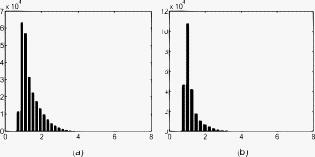
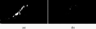
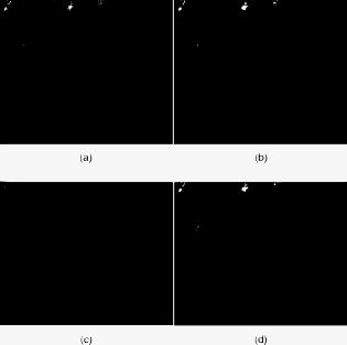
Let us now concentrate on estimation of noise local SD in the spectral (DCT) domain. For a given block, it is possible to estimate in a spectral domain as39, 48 where med{ } denotes the median of a data sample. This estimate is similar to the median of absolute deviations used as a robust data scale estimator.9 Here [in Eq. 8], the noise SD (scale) estimate exploits properties of transform coefficients when mixed Gaussian–Laplacian or Gaussian scale mixture models for their description are used.54 Two properties of orthogonal transforms and robust estimation are exploited in Eq. 8. First, noise after an orthogonal transform spreads between all coefficients, and, if noise is independent identically distributed (i.i.d), its power spreads uniformly where spectral coefficients occur to be Gaussian random variables. Then, the SD of spectral coefficients is proportional to the noise SD. Second, the use of the robust estimate (median) provides less sensitivity to outliers where the outliers in the considered case are induced by image content.However, although the used estimator (sample median) is robust, the image local content (details, texture, edges) present in a given block leads to the positive bias of the estimate .52 Note that if noise is spatially correlated, considerable bias can be observed for estimates obtained according to Eq. 651 (these estimates in homogeneous regions are, on average, smaller than the true value of noise SD). Let us analyze how great the influence of image local content and other factors could be on accuracy of local estimates. Consider a test image [e.g., the standard test image Barbara, (Fig. 2 )] corrupted by white additive noise with a zero mean and constant variance . The values of from Eq. 6 are visualized in Fig. 2; larger values are lighter (magnification by 7 is used for better visualization). It is seen that the values for blocks that correspond to homogeneous image regions vary a little. They are mostly rather small and approximately equal to of additive noise. The values for the blocks that correspond to image heterogeneities such as edges, textures, and details, are commonly slightly larger due to influence of image content. Fig. 2(a) Noise-free test image Barbara, (b) visualized of test image Barbara (values have been multiplied by 7) and (c) (values have been multiplied by 3.5). 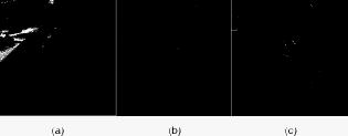 Behavior of is similar [see Fig. 2 magnification is by 3.5], but its sensitivity to image heterogeneities in blocks is considerably larger. This can be also seen from the comparison of histograms of and presented in Figs. 3 and 3 respectively. In both cases, normal local estimates (which are obtained in homogeneous image blocks) are grouped near the true value equal to 10. But for the histogram in Fig. 3 there are more abnormal local estimates and they are, on average, larger. This analysis allows proposing a locally adaptive DCT-based filter that will be further referred as LA DCT-1. This filter algorithm is as follows: We prefer to use , but not , because is less sensitive to heterogeneities. Note that the use of a larger threshold in DCT-based filtering leads to oversmoothing. As follows from the algorithm description, the proposed filter LA DCT-1 adapts to noise local characteristics. This is adaptation mechanism 1.3.2.Improved Locally Adaptive DCT FilterIn this section, we consider one more way (mechanism 2) to further improve performance of the locally adaptive DCT-based filter. Our approach is based on the following general idea and assumptions. Suppose that we have succeeded in discriminating homogeneous and heterogeneous regions of an image. Because in homogeneous regions, local estimates are quite close to true values of local SD of noise, then it is a correct decision to set the local threshold equal to . On the contrary, if a given block corresponds to an image heterogeneous region, then, most probably, is larger than the local SD of noise. Then, it is reasonable to set the local threshold less than as , where . In general, there are many possible ways to set . It can be fixed and equal to some in a simplest case or it can be determined in a more complicated manner. Thus, a primordial task is to design some discriminator for homogeneous and heterogeneous blocks. It is easy to resolve this task if one knows the local SD of noise in advance.7 However, it becomes more complicated if the local SD of nonstationary noise is unknown. To get around this shortcoming, let us exploit the properties of local estimates (in spectral domain) and (in spatial domain) established in Section 3.1. Note that usually7 is defined in square-shaped scanning windows, where window side size is odd (e.g., 5 or 7).7, 23 Because here we deal with DCT-based filtering in blocks, it is possible to calculate either according to Eq. 6 or as follows: The map of the estimates for is visualized in Fig. 2 for the test image Barbara corrupted by zero mean additive noise with the constant variance . Because the estimate is much more sensitive to image heterogeneities in a block than the estimate , let us exploit this difference for discriminating homogeneous and heterogeneous image blocks. For this purpose, consider a ratio . Its example for the test image Barbara and additive Gaussian noise with is visualized in Fig. 4 . We represent the ratio map as an image , , , where [•] means rounding to the nearest positive integer not larger than 255, is the image size, 40 is a magnification coefficient used to visualize better the maps .Fig. 4Magnified ratio image for the test image Barbara (a) corrupted by additive noise and (b) corrupted by Poisson noise.  Joint visual analysis of the test image Barbara [Fig. 2] and the ratio map [Fig. 4] shows that quite large ratios (essentially larger than unity, indicated by brighter color pixels) are observed for blocks located in the heterogeneous image regions. Figure 4 presents the ratio map for the same test image but corrupted by Poisson noise. The obtained maps are rather similar. This indicates that the method of analyzing local activity (heterogeneity) based on is applicable to different types of noise. This observation allows expectation that the proposed principle will also work well enough for any nonstationary noise. There are several possible ways to exploit the aforementioned property. The simplest one is to adaptively set the local threshold where as in LA DCT-1, is a preset threshold, is a factor that determines the hard threshold for DCT coefficients in edge/detail neighborhoods and in textural regions. The DCT-based filter described by Eqs. 5, 9, 10 (further referred as to LA DCT-2) belongs to the class of locally adaptive hard-switching filters,7 where hard switching relates to the parameter . This filter implies both adaptions to noise characteristics (mechanism 1) and to image content (mechanism 2).LA DCT-2 uses two new parameters, and . Consider distributions of the ratio , which is a random variable. Suppose that the estimates and are obtained in a homogeneous image region. Then, their means under condition of i.i.d. Gaussian noise are the same. Thus, it is possible to expect that the distribution of the ratio should have a mode in the neighborhood of unity. As follows from the ratio maps in Figs. 4 and 4, is usually larger than in image heterogeneous regions. Therefore, the distribution of the ratio may have a heavy “right-hand” tail. The histogram of the obtained values for the test image Barbara (pure additive Gaussian noise, ) is presented in Fig. 5 . The histogram for the image Lenna corrupted by Poisson noise is shown in Fig. 5. Both distributions, as expected, have modes in the neighborhoods of unity, and they possess a heavy right-hand tail. Similar shapes of value distributions have been observed for other conventional test images as Peppers, Goldhill, etc. The detailed analysis of values of these histograms shows that the distribution mode, which corresponds to homogeneous image regions, is about unity. Being random, the values form the quasi-Gaussian part of this distribution. As in any discrimination or detection task, a larger preset discrimination threshold provides better correct detection of homogeneous regions but larger probability of recognizing heterogeneous region as homogeneous. Thus, threshold setting is a compromise. Analysis of histogram data shows that a trade-off in discriminating blocks that correspond to homogeneous and heterogeneous regions can be provided by setting . 4.Local Adaptive DCT Filter Performance Analysis4.1.Performance Analysis for Test Images in Case of Spatially Uncorrelated NoiseLet us carry experiments with different types of noise and test images. Recall that if noise type and characteristics are a priori known, it is possible to carry out filtering in a priori adjusted or “ideal” manner. For example, if one knows that noise is additive with fixed , then it is possible to apply the standard DCT-based filter31 with the fixed . Similarly, if, e.g., noise is Poissonian, filtering can be done with (see Section 2). Quantitative performance characteristics for such filters that presume availability of full a priori information and its use, IdDCT, can serve as benchmarks of what can be reached if a priori information is available and is exploited in the DCT-based filtering. Let us analyze the filter performance in conventional terms of output where MSE is mean square error, is the image size, is the ’th pixel value for the processed (filtered) image. The simulation results have been obtained for the traditional set of test gray-scale images , for Gaussian additive and Poisson noises. These simulation results are collected in Table 1 . Two values of have been used, namely, and 2.3 as motivated by dependences in Fig. 1 and analysis performed in Sections 2, 3. Table 1Output MSE for “ideal” DCT-based (IdDCT) filter, LA DCT-1, and nonlinear nonadaptive filters.
Table 1 also contains the values of for four nonadaptive nonlinear filters: the standard median with the scanning window sizes and , the -trimmed mean (ATM) filter with trimmed two largest and two smallest values in the scanning window, and the center-weighted median (CWM) filter with the central pixel weight equal to 3.23 Analysis of data in Table 1 shows the following:
Table 2Values of MSEout for several βhet and TR for the considered test images.
As follows from analysis of the obtained results, for most images it is reasonable to set , . This choice produces falling into the neighborhood of minimal for both noise models and for the four considered test images. The only exception is the test image Baboon, for which it is reasonable to use smaller . Reduction of by approximately 10–30% is observed for LA DCT-2 in comparison to LA DCT-1 with fixed (compare the data in Tables 1, 2). Improvement in comparison to LA DCT-1 with fixed is larger for more complex images. The values of are almost the same as were observed for the IdDCT filter. Only for test image Baboon are the results not good enough. We have examined the a reason for this. It occurred that the values in image texture regions are about four times larger than the true values of local SD of noise . Thus, even if is set to , the local threshold is larger than . Because of this, some oversmoothing takes place even for LA DCT-2. In addition to hard switching of according to Eq. 10, we have also analyzed another (soft) algorithm of threshold adaptation as follows: We have tested this method for the same test images and noise models as presented in Table 2. Very similar results as for the LA DCT-2 with optimally set , have been obtained. One reason why it is difficult to improve performance of the locally adaptive DCT-based filters is that there are many blocks for which the ratio is close to unity although these blocks are, in fact, heterogeneous. This means that, in the future, it is worth studying other local parameters than that should be able to better discriminate homogeneous and heterogeneous image blocks. In particular, gaussianity tests in spatial or spectral domain are worth studying.55Let us compare the data obtained for LA DCT-2 to other locally adaptive filters. The best known results of removing noise with a priori unknown characteristics are presented in the paper of Kervrann and Boulanger,26 who perform a thorough comparison of their method to other filtering methods and demonstrate superior performance of their approach. Thus, we present our results obtained for the recommended , and Kervrann and Boulanger’s data for the same test images and noise variances (Table 3 ). Noise is additive white Gaussian. Filter performance is characterized by output PSNR. Table 3PSNR for the compared LA-DCT-2 and Kervrann’s filters.
As is seen, the method26 produces slightly better results for larger noise variance and simpler test images. In turn, our method LA DCT-2 provides larger PSNR for smaller SD of noise and more textural images. The advantage of the proposed method LA DCT-2 is that image processing is quite fast. This is due to the fact that two basic operations used in the proposed techniques are DCT and data sorting where both can be realized using fast algorithms.42 4.2.Filter Performance in Spatially Correlated Noise EnvironmentThe case of spatially uncorrelated (i.i.d.) noise has been studied. However, in practice, it is possible that noise can be spatially correlated. Furthermore, 2-D autocorrelation function of spatially correlated noise can be unknown in advance.7, 51 We have analyzed how the proposed LA DCT-2 filter performs in the situation of spatially correlated noise. For this purpose, we have simulated additive Gaussian zero mean spatially correlated noise with variance 100. Spatially correlated noise has been modeled by applying the window mean filter to originally i.i.d. zero mean Gaussian 2-D noise and adjusting a desired variance. The results are presented in Table 4 for three values of and several values of . The test images are the same as earlier. Table 4Values of MSEout for several βhet and TR for the considered test images corrupted by spatially correlated noise.
Analysis of the data presented in Table 4 shows the following:
Another reason is that statistical characteristics of and as well as their ratio change if noise is spatially correlated with respect to the i.i.d. noise case. Let us analyze histograms of for spatially correlated noise. Two typical histograms are presented in Fig. 6 . Their shapes are similar to the shapes of the histograms represented in Fig. 5. However, there is an obvious difference. The modes of the histograms in Fig. 6 occur not in the neighborhood of unity but for larger values. Fig. 6Histograms of the ratio for the test images: (a) Lenna and (b) Barbara corrupted by zero mean spatially correlated additive Gaussian noise with . 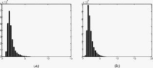 This phenomenon has its explanation. For spatially correlated noise, both estimates and in homogeneous blocks (that form histogram maximum) become biased, smaller than the true value of noise SD.51 But the bias of the estimates can be about , whereas for the estimates the bias can reach .51 Thus, the estimates in image homogeneous blocks are, on average, larger than the estimates . This leads to mode shifting to values larger than unity. Let us analyze the mode estimates for distributions of . The obtained data are presented in Table 5 . The method49 has been applied for mode estimation. Table 5Estimates r̂ for the test images corrupted by different types of noise.
As is seen, for spatially uncorrelated noise the estimates are quite close to unity for all test images for both additive i.i.d. Gaussian and Poissonian noise. One interesting observation is that, for images with more complicated structure (e.g., Baboon), the estimates are larger. Similarly, if noise is spatially correlated, the estimates are considerably larger than 1.0 for all five considered test images. Two conclusions follow from this analysis:
5.Performance Analysis for Real-Life ImagesLet us present two examples of applying the proposed filters to real-life data. One example is a set of polarimetric radar data, presented as real valued (floating point) data arrays. These data have been obtained by a maritime coastal radar. The images are presented in Fig. 7 . HH means that a horizontally polarized signal is transmitted and then received; VH relates to a vertically polarized emitted and horizontally polarized received signal. A sensed area mainly corresponds to sea surface (that occupies basic part of images and form background), one large rock (small rocky island placed in the image central part, very bright pixels), several small ones (left lower corner, groups of bright pixels), and a shadowed zone behind the large rock. The horizontal axis of images corresponds to range and vertical axis relates to azimuth of the radar. During data acquisition, internal gain control was used to partly compensate dependence of backscattered signal mean on distance. Visual analysis of these images allows concluding that background intensity varies depending on range. More detailed analysis has been done to confirm this conclusion. First, histograms (Fig. 8 ) have been obtained for manually selected six “homogeneous” regions (marked by frames in images in Fig. 7) for two different sectors and three different mean distances. Analysis of sample histograms in Fig. 8 shows that the histogram shape changes with range. The distributions are asymmetric with respect to their means. There is a heavy tail to the right side from the distribution mode. Distribution modes are also different for different ranges. Outliers are seldom (occur with quite small probabilities), their values differ from the mode values by approximately ten times. Fig. 8Sample histograms for the image in Fig. 7 (a) for small distance fragment 1 and (b) for middle distance fragment 3.  To carry out more thorough analysis, we have determined the following parameters for each image homogeneous region:
The results obtained for the image in Fig. 7 are given in Table 6 . For more distant fragments (5 and 6), the values and are larger than for less distant fragments, especially for the fragments 1 and 2. In turn, the standard and robust (interquantile) estimates of relative variance for more distant fragments are smaller. This shows that noise is neither pure additive nor pure multiplicative. A specific “distance-dependent” noise is observed. This conclusion has been confirmed by results of analysis carried out for the image in Fig. 7. The observed nonstationarity results from joint influence of several factors, namely, specific features of the receiver amplifier gain control used, varying incidence (grazing) angle of backscattering from wavy sea surface, different mutual geometry of sea wave direction and radar azimuth, etc. This is the case when it is difficult to separate the influence of these factors. We assume that nonstationary noise local statistics does not change abruptly [i.e., it is possible to consider it practically constant for fragments (blocks) of relatively small size, let us say blocks commonly used in DCT-based filtering]. Table 6Statistical characteristics of the selected “homogeneous” regions for the image in Fig. 7.
Figure 9 presents the processed images for the maritime radar data carlier given in Fig. 8. Note that in this case, a two-stage procedure has been applied. At the first stage, the CW Median filter23 with the scanning window and the center element weight has been used to remove outliers. Then, at the second stage, the LA DCT-1 has been used. Comparing images in Figs. 7 and 9, one can conclude that noise is well suppressed and useful information in images is preserved well enough, although some oversmoothing of fine details is observed. Let us give another example of a real-life image processing. The 224th subband image of the Lunar Lake AVIRIS57, 58, 59 image is presented in Fig. 10 . Noise present in this image is visually seen. The output image for LA DCT-1 is shown in Fig. 10. Noise is well suppressed, although sharp edges are slightly smeared. The ratio image is visualized in Fig. 10. The most sharp edges and details are marked by brighter color pixels in this map. This allows better preservation of sharp edges and details in the output image by the designed LA DCT-2 [see Fig. 10 , , ]. 6.Conclusions and Future WorkIt is shown that there are practical situations where noise is nonstationary and limited a priori information on its statistics is available. To filter images effectively under these conditions, two DCT-based filtering techniques to suppress nonstationary spatially uncorrelated noise have been proposed and studied. The first technique is a locally adaptive filter based on local estimation of noise variance in blocks and setting the corresponding threshold proportionally to the obtained estimate of noise SD. It performs well enough for rather simple images. The second locally adaptive filter employs, in addition, the analysis of the ratio and adapts to image content in a block. This leads to decreasing and improving edge/detail/texture preservation in processed images. As a result, the performance of this filter is comparable to performance of the best state-of-the-art methods. The recommendations concerning proper selection of the filter adaptation parameters are given. The designed filters have been applied to real-life images and have demonstrated excellent results. The spatially correlated noise case has been studied as well. The proposed methods do not perform well enough for this case and should be further modified. A way to discriminate the cases of spatially uncorrelated and correlated noise has been proposed. The design of locally adaptive filters for spatially correlated noise case may be a subject of our future work. AcknowledgmentsWe are thankful to anonymous reviewers for their valuable comments and propositions. The work of O. Pogrebnyak was partially supported by Instituto Politecnico Nacional as a part of the research project SIP No. 20101090. Images have been kindly provided by Dr. A.V. Popov, of National Aerospace University, Kharkov, Ukraine. referencesP.-L. Shui,
“Image denoising algorithm via doubly local wiener filtering with directional windows in wavelet domain,”
IEEE Signal Process. Lett., 12
(10), 681
–684
(2005). https://doi.org/10.1109/LSP.2005.855555 Google Scholar
A. Foi, V. Katkovnik, and K. Egiazarian,
“Signal-dependent noise removal in point-wise shape-adaptive DCT domain with locally adaptive variance,”
(2007). Google Scholar
S. Solbo and T. Eltoft,
“Homomorphic wavelet-based statistical despeckling of SAR images,”
IEEE Trans. Geosci. Remote Sens., 42
(4), 711
–721
(2004). https://doi.org/10.1109/TGRS.2003.821885 Google Scholar
H.-L. Eng and K.-K. Ma,
“Noise adaptive soft switching median filter,”
IEEE Trans. Image Process., 10
(2), 242
–251
(2001). https://doi.org/10.1109/83.902289 Google Scholar
Nonlinear Signal and Image Processing: Theory, Methods, and Applications, CRC Press, Boca Raton
(2003). Google Scholar
K. N. Plataniotis and A. N. Venetsanopoulos, Color Image Processing and Applications, Springer-Verlag, New York
(2000). Google Scholar
V. Melnik,
“Nonlinear locally adaptive techniques for image filtering and restoration in mixed noise environments,”
Tampere University of Technology,
(2000). http://www.atilim.edu.tr/~roktem/Research/interests.htm Google Scholar
V. V. Lukin, N. N. Ponomarenko, S. K. Abramov, B. Vozel, K. Chehdi, and J. Astola,
“Filtering of radar images based on blind evaluation of noise characteristics,”
Proc. SPIE, 7109 71090R
(2008). https://doi.org/10.1117/12.799396 Google Scholar
J. Astola and P. Kuosmanen, Fundamentals of Nonlinear Digital Filtering, CRC Press, Boca Raton, FL
(1997). Google Scholar
R. Touzi,
“A review of speckle filtering in the context of estimation theory,”
IEEE Trans. Geosci. Remote Sens., 40
(11), 2392
–2404
(2002). https://doi.org/10.1109/TGRS.2002.803727 Google Scholar
D. K. Barton, Radar System Analysis and Modeling, Artech House, Boston
(2005). Google Scholar
G. P. Kulemin, A. A. Zelensky, J. T. Astola, V. V. Lukin, K. O. Egiazarian, A. A. Kurekin, N. N. Ponomarenko, S. K. Abramov, O. V. Tsymbal, Y. A. Goroshko, and Y. V. Tarnavsky, Methods and Algorithms for Pre-processing and Classification of Multichannel Radar Remote Sensing Images, TTY Monistamo, Tampere, Finland
(2004). Google Scholar
C. Lopez-Martinez and E. Pottier,
“On the extension of multidimensional speckle noise model from single-look to multilook SAR imagery,”
IEEE Trans. Geosci. Remote Sens., 45
(2), 305
–320
(2007). https://doi.org/10.1109/TGRS.2006.887012 Google Scholar
Hyperspectral Data Exploitation: Theory and Applications, Wiley, Hoboken, NJ
(2007). Google Scholar
R. Lukac, K. N. Plataniotis, B. Smolka, and A. N. Venetsanopoulos,
“cDNA microarray image processing using fuzzy vector filtering framework,”
J. Fuzzy Sets Syst., 152
(1), 17
–35
(2005). https://doi.org/10.1016/j.fss.2004.10.012 Google Scholar
G. P. Kulemin, Millimeter-Wave Radar Targets and Clutter, Artech House, Boston
(2003). Google Scholar
C. Oliver and S. Quegan, Understanding Synthetic Aperture Radar Images, SciTech Publishing, Raleigh, NC
(2004). Google Scholar
J. S. Lee, J. H. Wen, T. I. Ainsworth, K. S. Chen, and A. J. Chen,
“Improved sigma filter for speckle filtering of SAR imagery,”
IEEE Trans. Geosci. Remote Sens., 47
(1), 202
–213
(2009). https://doi.org/10.1109/TGRS.2008.2002881 Google Scholar
A. Barducci, D. Guzzi, P. Marcoionni, and I. Pippi,
“CHRIS-Proba performance evaluation: signal-to-noise ratio, instrument efficiency and data quality from acquisitions over San Rossore (Italy) test site,”
(2005). Google Scholar
P. Koivisto, J. Astola, V. Lukin, V. Melnik, and O. Tsymbal,
“Removing impulse bursts from images by training based filtering,”
EURASIP J. Appl. Signal Process., 2003
(3), 223
–237
(2003). https://doi.org/10.1155/S1110865703211045 Google Scholar
T. Rabic,
“Robust estimation approach to blind denoising,”
IEEE Trans. Image Process., 14
(11), 1755
–1766
(2005). https://doi.org/10.1109/TIP.2005.857276 Google Scholar
P. Huber, Robust Statistics, Wiley, Hoboken, NJ
(1981). Google Scholar
T. Sun, M. Gabbouj, and Y. Neuvo,
“Center weighted median filters: some properties and their applications in image processing,”
Signal Process., 35
(3), 213
–229
(1994). https://doi.org/10.1016/0165-1684(94)90212-7 Google Scholar
O. V. Tsymbal, V. V. Lukin, N. N. Ponomarenko, A. A. Zelensky, K. O. Egiazarian, and J. T. Astola,
“Three-state locally adaptive texture preserving filter for radar and optical image processing,”
EURASIP J. Appl. Signal Process., 8 1185
–1204
(2005). Google Scholar
L. P. Yaroslavsky,
“Local criteria and local adaptive filtering in image processing: a retrospective view,”
(2008). Google Scholar
C. Kervrann and J. Boulanger,
“Local adaptivity to variable smoothness for exemplar-based image regularization and representation,”
Int. J. Comput. Vis., 79
(1), 45
–69
(2008). https://doi.org/10.1007/s11263-007-0096-2 Google Scholar
P. Perona and J. Malik,
“Scale space and edge detection using anisotropic diffusion,”
IEEE Trans. Pattern Anal. Mach. Intell., 12
(7), 629
–639
(1990). https://doi.org/10.1109/34.56205 Google Scholar
L. Rudin, S. Osher, and E. Fatemi,
“Nonlinear total variation based noise removal algorithms,”
Physica D, 60 259
–268
(1992). https://doi.org/10.1016/0167-2789(92)90242-F Google Scholar
V. G. Spokoiny,
“Estimation of a function with discontinuities via local polynomial fit with an adaptive window choice,”
Ann. Stat., 26
(4), 141
–170
(1998). Google Scholar
S. Mallat, A Wavelet Tour of Signal Processing, Academic Press, San Diego
(1998). Google Scholar
V. V. Lukin, R. Oktem, N. Ponomarenko, and K. Egiazarian,
“Image
filtering based on discrete cosine transform,”
Telecommun. Radio Eng., 66
(18), 1685
–1701
(2007). https://doi.org/10.1615/TelecomRadEng.v66.i18.70 Google Scholar
M. C. Motwani, M. C. Gadiya, R. C. Motwani, and F. C. Harris,
“Survey of image denoising techniques,”
(2004). Google Scholar
R. Oktem, K. Egiazarian, V. Lukin, N. Ponomarenko, and O. Tsymbal,
“Locally adaptive DCT filtering for signal-dependent noise removal,”
EURASIP J. Adv. Signal Process., 2007 42472
(2007). https://doi.org/10.1155/2007/42472 Google Scholar
L. Klaine, B. Vozel, and K. Chehdi,
“An integro differential method for adaptive filtering of additive or multiplicative noise,”
1001
–1004
(2005). Google Scholar
F. Argenti, G. Torricelli, and L. Alparone,
“Signal dependent noise removal in the undecimated wavelet domain,”
3293
–3296
(2002). Google Scholar
A. Foi,
“Pointwise shape-adaptive DCT image filtering and signal-dependent noise estimation,”
Tampere University of Technology,
(2007). Google Scholar
R. Oktem,
“Transform domain algorithms for image compression and denoising,”
Tampere University of Technology,
(2000). Google Scholar
L. Sendur and I. W. Selesnick,
“Bivariate shrinkage with local variance estimation,”
IEEE Signal Process. Lett., 9
(12), 438
–441
(2002). https://doi.org/10.1109/LSP.2002.806054 Google Scholar
D. V. Fevralev, V. V. Lukin, A. V. Totsky, K. Egiazarian, and J. Astola,
“Combined bispectrum filtering technique for signal shape estimation with DCT based adaptive filter,”
133
–140
(2006). Google Scholar
R. Coifman and D. L. Donoho,
“Translation invariant denoising,”
Wavelets and Statistics, Springer-Verlag, Berlin
(1995). Google Scholar
D. Salomon, Data Compression: The Complete Reference, Springer, New York
(2007). Google Scholar
L. P. Yaroslavsky, Digital Holography and Digital Image Processing: Principles, Methods, Algorithms, Kluwer, Dordrecht
(2004). Google Scholar
H. Huang, X. Lin, S. Rahardja, and R. Yu,
“A method for realizing reversible type-IV discrete cosine transform (IntDCT-IV),”
101
–104
(2004). Google Scholar
G. Wallace,
“JPEG still image compression standard,”
Commun. ACM, 34
(4), 30
–44
(1991). https://doi.org/10.1145/103085.103089 Google Scholar
A. Bovik, Handbook on Image and Video Processing, Academic Press, New York
(2000). Google Scholar
N. Ponomarenko, V. Lukin, A. A. Zelensky, J. Astola, and K. Egiazarian,
“Adaptive DCT-based filtering of images corrupted by spatially correlated noise,”
Proc. SPIE, 6812 68120W
(2008). https://doi.org/10.1117/12.764893 Google Scholar
V. V. Lukin, D. V. Fevralev, S. K. Abramov, S. Peltonen, and J. Astola,
“Adaptive DCT-based 1-D filtering of Poisson and mixed Poisson and impulsive noise,”
(2008). Google Scholar
V. V. Lukin, D. V. Fevralev, N. N. Ponomarenko, O. B. Pogrebnyak, K. O. Egiazarian, and J. T. Astola,
“Local adaptive filtering of images corrupted by nonstationary noise,”
Proc. SPIE, 7245 724506
(2009). https://doi.org/10.1117/12.805298 Google Scholar
V. V. Lukin, S. K. Abramov, A. A. Zelensky, J. Astola, B. Vozel, and B. Chehdi,
“Improved minimal interquantile distance method for blind estimation of noise variance in images,”
Proc. SPIE, 6748 67481I
(2007). https://doi.org/10.1117/12.738006 Google Scholar
V. V. Lukin, P. T. Koivisto, N. N. Ponomarenko, S. K. Abramov, and J. T. Astola,
“Two-stage methods for mixed noise removal,”
(2005). Google Scholar
S. Abramov, V. Lukin, B. Vozel, K. Chehdi, and J. Astola,
“Segmentation-based method for blind evaluation of noise variance in images,”
J. Appl. Remote Sens., 2 023533
(2008). https://doi.org/10.1117/1.2977788 Google Scholar
N. N. Ponomarenko, V. V. Lukin, S. K. Abramov, K. O. Egiazarian, and J. T. Astola,
“Blind evaluation of additive noise variance in textured images by nonlinear processing of block DCT coefficients,”
Proc. SPIE, 5014 178
–189
(2003). https://doi.org/10.1117/12.477717 Google Scholar
C. Liu, R. Szeliski, S. B. Kang, C. L. Zitnick, and W. T. Freeman,
“Automatic estimation and removal of noise from a single image,”
IEEE Trans. Pattern Anal. Mach. Intell., 30
(2), 299
–314
(2008). https://doi.org/10.1109/TPAMI.2007.1176 Google Scholar
J. Portilla, V. Strela, M. Wainwright, and E. P. Simoncelli,
“Image denoising using Gaussian scale mixtures in the wavelet domain,”
IEEE Trans. Image Process., 12
(11), 1338
–1351
(2003). https://doi.org/10.1109/TIP.2003.818640 Google Scholar
N. Ponomarenko, D. Fevralev, A. Roenko, S. Krivenko, V. Lukin, and I. Djurovic,
“Edge detection and filtering of images corrupted by nonstationary noise using robust statistics,”
129
–136
(2009). Google Scholar
N. Ponomarenko, V. Lukin, I. Djurovic, and M. Simeunovic,
“Pre-filtering of multichannel remote sensing data for agricultural bare soil field parameter estimation,”
(2009). Google Scholar
N. Ponomarenko, V. Lukin, M. Zriakhov, and A. Kaarna,
“Preliminary automatic analysis of characteristics of hyperspectral AVIRIS images,”
158
–160
(2006). Google Scholar
E. Christophe, D. Leger, and C. Mailhes,
“Quality criteria benchmark for hyperspectral imagery,”
IEEE Trans. Geosci. Remote Sens., 43
(9), 2103
–2114
(2005). https://doi.org/10.1109/TGRS.2005.853931 Google Scholar
Biography Vladimir V. Lukin graduated from Kharkov Aviation Institute (now National Aerospace University) in 1983, with his Diploma with honor in radio engineering. Since then he has been with the Department of Transmitters, Receivers and Signal Processing at National Aerospace University. He defended the thesis of Candidate of Technical Science in 1988 and Doctor of Technical Science in 2002 in DSP for remote sensing. Since 1995, he has been in cooperation with Tampere University of Technology. Currently, he is department vice-chairman and professor. His research interests include digital signal/image processing, remote sensing data processing, image filtering, and compression.  Dmitriy V. Fevralev graduated from National Aerospace University in 2002 with a Diploma in radio engineering. Since then he has been with the Department of Transmitters, Receivers and Signal Processing at National Aerospace University. He defended his thesis of Candidate of Technical Science in 2008 in DSP for bispectral analysis in radar systems. Currently, he is research fellow and part-time assistant with the Department of Transmitters, Receivers and Signal Processing. His research interests include digital signal/image processing, bispectral analysis of radar signals, and image filtering.  Nikolay N. Ponomarenko graduated from National Aerospace University in 1995 and received his Diploma with honor in computer science. Since then he has been with the Department of Transmitters, Receivers and Signal Processing at National Aerospace University. He defended his thesis of Candidate of Technical Science in 2004 in DSP for remote sensing. He also defended his thesis of Doctor of Technology at Tampere University of Technology, Finland, in 2005, on image compression. Currently, he is senior researcher and part-time associate professor with the Department of Transmitters, Receivers and Signal Processing. His research interests include digital signal/image processing, remote sensing data processing, image filtering, and compression.  Sergey K. Abramov graduated from National Aerospace University in 2000 with a Diploma with honor in radio engineering. Since then, he has been with the Department of Transmitters, Receivers and Signal Processing at National Aerospace University. He defended his thesis of Candidate of Technical Science in 2003 in DSP for remote sensing. Currently, he is associate professor and part-time senior researcher with the Department of Transmitters, Receivers and Signal Processing. His research interests include digital signal/image processing, blind estimation of noise characteristics, and image filtering.  Oleksiy Pogrebnyak received his Ph.D. degree from Kharkov Aviation Institute (now National Aerospace University), Ukraine, in 1991. Currently, he is with The Center for Computing Research of National Polytechnic Institute, Mexico. His research interests include digital signal/image filtering and compression and remote sensing.  Karen O. Egiazarian received her PhD from Moscow M. V. Lomonosov State University, Russia, in 1986, and Doctor of Technology degree from Tampere University of Technology, Finland, in 1994. He is a leading scientist in signal, image, and video processing, with about 300 refereed journal and conference articles, three book chapters, and a book published by Marcel Dekker. His main interests are in the field of multirate signal processing, image and video denoising and compression, and digital logic. He is a member of the DSP Technical Committee of the IEEE Circuits and Systems Society.  Jaakko Astola received his BS, MS, Licentiate, and PhD in mathematics from Turku University, Finland, in 1972, 1973, 1975, and 1978, respectively. From 1976 to 1977, he was with the Research Institute for Mathematical Sciences of Kyoto University, Kyoto, Japan. Since 1979 to 1987, he was with Lappeenranta University of Tecvhnology (Finland). From 1987, he is with Tampere University of Technology, Tampere, Finland. Currently, he is professor of signal processing and director of Tampere International Center for Signal Processing, academy professor by the Academy of Finland, and IEEE fellow. His research interests include signal/image processing, statistics, and image coding. |
||||||||||||||||||||||||||||||||||||||||||||||||||||||||||||||||||||||||||||||||||||||||||||||||||||||||||||||||||||||||||||||||||||||||||||||||||||||||||||||||||||||||||||||||||||||||||||||||||||||||||||||||||||||||||||||||||||||||||||||||||||||||||||||||||||||||||||||||||||||||||||||||||||||||||||||||||||||||||||||||||||||||||||||||||||||||||||||||||||||||||||||||||||||||||||||||||||||||||||||||||||||||||||||||||||||||||||||||||||||||||||||||||||||||||||||||||||||||||||||||||||||||||||||||||||||||||||||||||||||||||||||||||||||||||||||||||||||||||||||||||||||||||||||||||||||||||||||||||||||||||||||||||||||||||||||||||||||||||||||||||||||||||||||||||||||||||||||||||||||||||||||||||||||||||||||||||||||||||||||||||||||||||||||